Techniques for cooling to ultralow temperatures
- Also see: Magnetic trapping and evaporative cooling (2009 Class Notes File:Magnetic trappping and evaporative cooling.pdf)
Magnetic confinement
The principle of magnetic trapping is deflection by magnetic fields. This is at the heart of the Stern-Gerlach experiment in 1925. In the 1960's it was realized that magnetic confinement could be realized. It was first realized for neutrons, in 1978 by Paul. The exciting 1980's was magnetic cooling and trapping, including work by Phillips, Pritchard, and Greytak, on sodium and other atoms.
Earnshaw theorem
Recall the Earnshaw theorem, previously discussed for the optical force, and for trapped ions. This states that trapping requires or . For a rigid charge distribution, with positions , where is the center of mass motion and is the relative position of charge , we find that
must satisfy . An arbitrary rigid charge distribution (with arbitrary multiple moments) cannot be kept in stable equilibrium at rest in free space in static electric fields. The same theorem applies for magnetic multipole distributions.
Circumventing the Earnshaw theorem
Sir James-Jeans, in 1925, pointed out a way around this limit. If the matter is polarizable, this can change the electric fields.
The displacement of the trapped particle or of the field generated by a particle which are energetically favorable are forbidden due to constraints. This leads to a loophole, as exemplified by magnet stabilized above a superconductor:
The constraint that no magnetic field may enter a superconductor causes shielding currents to be created which stabilize the trapping configuration for the levitated particle. This happens in a configuration which is not a minimum of the magnetic energies.
Of course, electronic feedback can be used to create a stable trapping potential, providing time varying fields.
Another example is provided by diamagnetic matter. Such matter expels an external field.
Yet another, important, example is if is constant. This constrains angular momentum; the dipole moment is not allowed to flip over to move into what might be a more energetically favorable configuration.
Trapping a magnetic moment
Now let us see how these ideas can allow trapping of an object with a magnetic moment. Let us consider when a magnetic moment might be constrained such that the potential depends only on the absolute value of the magnetic field, .
Wing's theorem
Wing's theorem (1983) says that in a region devoid of charges and currents, quasistatic electric of magnetic fields can have local minima, but not local maxima. The proof of this fact is by non-existence of a maximum by contradiction. Assume is a max. Then
It follows that
and the cross-term must be always negative. Without loss of generality, this requires, for example, . However, that presents a contradiction with the Laplace equation (recall Earnshaw's theorem). A minimum, on the other hand, is possible because of the term. There can thus be local minima, but not local maxima, in an electric field configuration.
By Wing's theorem, since there can only be local minima (and not maxima) in a static magnetic field, to have a stable magnetic trap, must be antiparallel to . The limits to stability of magnetic traps include spin relaxation (involving nuclear magnetic moment changes), dipolar relaxation (involving angular momenta changes of atomic motion), and Majorana flops.
Classical magnetic moment in a trap
More specifically, to trap, must be antiparallel to only adiabatically, as follows. Consider the problem of trapping a classical magnetic moment. Such a magnetic moment precesses in a magnetic field:
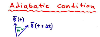
What is needed is for the precession of the magnetic moment to follow and maintain the same angle with respect to the field, as the moment moves in an inhomogeneous field. If the field changes slowly, the precession will follow the field, but if the field changes too rapidly, the spin may no longer be antiparallel with respect to the field:
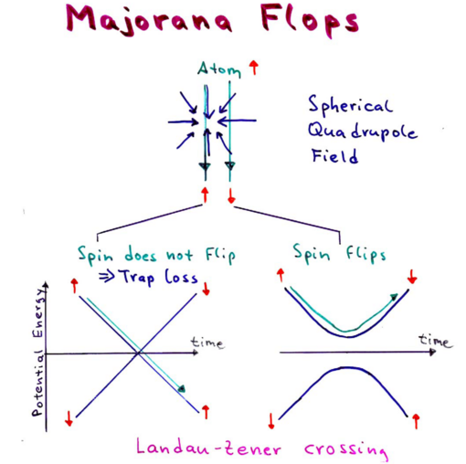
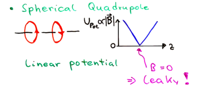
In the spherical quadrupole magnetic trap, made by anti-Helmholz coils, spins can flip in the following way, known as Majorana flops. As an atom moves through the field configuration:
it should flip its moment as it moves through the center of the field; however, there is a zero in the field at the center, at which point the spin can easily find itself aligned parallel with the field upon the atom's exit. This causes atoms to leak from the trap.
Levitron example
Counter-intuitively, spinning the top faster does not lead to a more stable trap. Rather, it causes increased instability; this is due to a process we may think of as being a classical analog of Majorana flops.
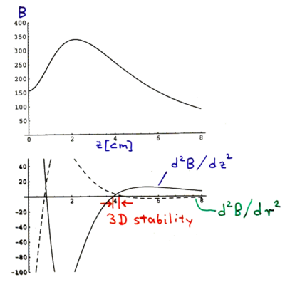
The levitron works in the following way. At ,
etc. The magnetic field above the center of the spinning magnet is thus
The second derviative of the magnetic field must give positive curvature along both the radial and axial directions, for the trap to be stable. This plot shows there is only a very small stability range for the trap.
Recall our trapping criterion: must stay anti-parallel to . This happens due to precession, as long as . The precession frequency of a gyroscope is given by the torque, so
where is the moment of inertia. is thus violated for large or . Around , one gets spin flips, referred to as Majorana flops in magnetic trapping of atoms.
Magnetic traps
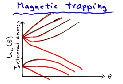
In magnetic traps, . can only have local minima, and not maxima, so we must ensure the angle of the field is such that the prefactors are positive. For Rubidium, we have these energy level dependencies on the field:
The only states which are trapped are thus which have positive energy versus magnetic field slope. The regimes with stable trapping are labeled with green in the above figure.
Magnetic traps can be separated into two broad categories: Those with a zero at the B-field minimum and those with a nonzero B-field minimum. We'll start by considering an example of the first type: the spherical quadrupole trap.
The spherical quadrupole trap can be generated from two coils with currents running in opposite directions. You may recognize this configuration as anti-Helmoltz coils, the same configuration used to generate the magnetic field for a MOT. This is depicted below.
Around the trap center the magnetic field components vary linearly with position
- Failed to parse (unknown function "\begin{align}"): {\displaystyle \begin{align} \ B_x &= B_x^\prime x \\ B_y &= B_y^\prime y \\ B_z &= B_z^\prime z \end{align} }
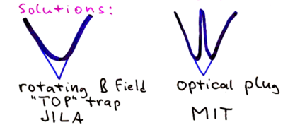
yielding the potential depicted in the figure above with a nice potential minimum to keep that atoms trapped. Unfortunately, the region where poses a problem. In order to stay trapped, the atom must stay in the correct Zeeman level, i.e. it must maintain its orientation with respect to its local magnetic field. As the atom moves around, the direction of the magnetic field changes and to stay trapped, the atom's orientation must adiabatically follow the magnetic field. Far from the center of the trap, this is no problem. The magnetic field changes direction slowly and smoothly so the atom rotates with it. However, an atom moving through the center of the trap sees the magnetic field get weaker until it suddenly flips direction and starts growing again. This sudden change causes the atom to change states to the opposite orientation with respect to the magnetic field. In other words, the atom changes to an anti-trapped state and is lost. This change from one state to another is called a Majorana flop, and the corresponding losses from a magnetic trap are called Majorana losses. A method is needed to plug the hole in the trap around the region.
One simple solution, which was the first used by BEC I at MIT is to superimpose a repulsive dipole trap using blue-detuned light over the trap center, thus repelling atoms from the region. Another idea is to use a time-dependent magnetic field as in a TOP trap, which was used for JILA's first BEC. The TOP trap adds a linear bias field to displace the bottom of the trap to one side. This linear bias field is then rapidly rotated, moving the minimum in a circle, such that the time-averaged orbiting potential (hence TOP) produces no zero in the magnetic field. Both of these techniques are depicted below
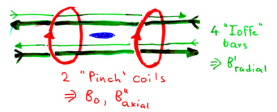
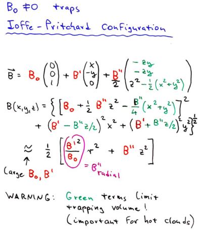
Another way to deal with the hole created by a region is to simply have a nonzero B-field minimum, which is the second type of traps mentioned above. In such traps the atoms can follow the magnetic field adiabatically, even as they pass through the trap center. A very popular trap that has this feature is the Ioffe-Pritchard trap, which was initially invented to confine plasmas, but actually works great for confining magnetically trapable atoms as well. The first part of an Ioffe-Pritchard provides axial confinement and consists of two "pinch" coils with currents running the same way in each to create a field minimum halfway between them with a nonzero magnetic field. The second part of the trap consists of four "Iofe" bars which produce a quadrupole trap that provides radial confinement. The geometry is depicted in the figure below.
The Ioffe bars create the quadrature field,
and the pinch field creates a linear field,
where the last term on the right is recognized to be . This configuration can be used with :
In practice the simple arrangement of wires described above is somewhat inconvenient for experiments because running the Ioffe bars through the vacuum chamber is a technical challenge. However the same magnetic trap (to leading order around the trap center) can be generated by wires arranged in a cloverleaf trap as depicted in the following photo.
The two pinch coils are visible on the left and the right depicts the four Ioffe bars which have been bent and wrapped into a circle.
Evaporative cooling
In the 1980s and 1990s laser cooling developments were able to push phase space densities to closer and closer to one, which is the threshold for Bose-Einstein condensation. However, as the cold atom clouds reached higher densities, laser cooling schemes hit an issue. When the atomic clouds were not too dense, each atom interacted with the laser field independently and cooling schemes that were designed to cool single atoms were able to cool clouds with multiple atoms. However, when the clouds became more dense, this was no longer the case. At high densities, atoms that entered an excited state while scattering a photon would interact strongly with a nearby atom. This would cause both atoms to fly out of the trap in a process called a light-assisted collision. This put a serious limit on the atomic densities that were achieved with laser cooling schemes. Therefore, atomic physicists wanted a final cooling technique to push their cold dense atomic clouds to condensation without scattering photons as in laser cooling schemes. This led to the development of a conceptually simple solution: evaporative cooling.
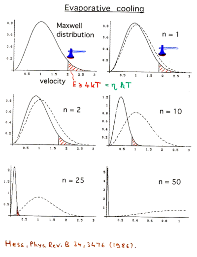
Evaporation allows cooling atoms to nanokelvin, or even subnanokelvin, temperatures even at high densities. It is the scheme that lead to the first BECs and remains a critical tool for nearly all degenerate gas experiments. To get a simple qualitative understanding for how it works, it's best to start by modeling the cooling as a series of discrete steps as in the figure below.
We start with a thermal cloud of atoms at a temperature , and then release all the atoms with energy greater that , where is an adjustable parameter of the cooling scheme. For this figure we've chosen . Since we've released the hottest atoms, the remaining atoms are have lower energy on average. We then wait for the cloud to thermalize and we're left with a gas that has fewer atoms and a colder temperature . The process then starts again now releasing all atoms with energy greater than . As the number for steps taken increases, the total atom number decreases, but the atomic velocities decrease, corresponding to a cooler cloud. This magnitude of this effect can be clearly seen by comparing the distributions to the initial distribution represented with a dashed line. In practice this process is not done by releasing the hottest atoms at discrete times. Instead the trap is adjusted to allow atoms with energy above a threshold energy to escape. This threshold energy can then be adjusted as the atoms evaporate to keep roughly constant.
Power Law Scalings
We see that evaporative cooling gives us the ability to trade atom number for lower temperatures. This begs the question, how good is this tradeoff? In the evaporative process a fraction of the atoms are traded for a fractional decrease of the temperature. This means that the relevant quantities are related by power laws and we should look at the derivatives of the logs of different quantities. For example, consider , the ratio of the fractional change in temperature to the fractional change in atom number, which therefore characterizes how efficient this atom-number-for-temperature trade is:
Now let's examine the case where the the trap potential is given by a power law
where is the number of dimensions and is chosen to give the correct scaling. For example, we'd have and for a harmonic trap in three dimensions. By the equipartition theorem, the kinetic energy and therefore temperature also scale the same way which we can invert to get . This leads to , and above we found that and so we can write . In this way we can write many interesting quantities of this system as power laws of with different exponents. The table below summarizes some results
| Quantity | Scaling Exponent | |
| Number of Atoms | ||
| Temperature | ||
| Volume | ||
| Number Density | ||
| Phase-Space Density | ||
| Elastic Collision Rate |
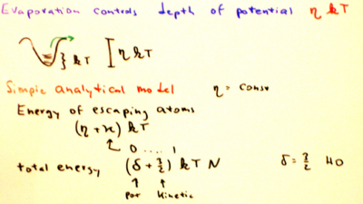
From this chart, the importance of is very clear; it characterizes all of the scalings for the thermodynamic quantities. Therefore we are interested in finding in terms of the experimentally controlled parameter . As depicted in the figure below, atoms with energy at least escape the trap, taking with them of energy with .
From the equipartition theorem, the total energy in the system is (assuming 3D motion). The total energy before and after the evaporation of atoms can then be related as (note that and are negative)
This can be rewritten as
Glancing back at the definition for above gives the result
Because the odds of an atom reaching a high energy state is exponentially suppressed, we can approximate that so that each atom takes of energy when it evaporates.
Speed of Evaporation
From this expression it seems that the evaporation can be arbitrarily efficient, just make as large as desired. The most extreme case of this would be to wait until one atom reaches so far into the high energy tail of the thermal distribution that it contains the entire energy of the system. In that case, simply evaporating one atom would leave the system at zero temperature. However, in practice extremely efficient evaporation like this is not feasible because the time necessary to evaporate increases with and the available time is limited due to other loss processes, such as background gas collisions, trap heating, or grad student life time. Therefore it is necessary to consider how quickly the evaporation takes place to determining the maximum achievable. To explore this further we examine the case of evaporation at constant and we'll neglect some factors on the order of unity that may come up when averaging over the full volume of the cloud, etc.
To determine the rate of evaporation we must calculate the rate at which collisions produce atoms with energy greater than . The simplest way to do this is to approximate and invoke the concept of detailed balance. Consider the velocity distribution of the atoms at the center of the trap of the trap where we take the potential energy to be zero, so that the atom's kinetic energy is equal to its total energy. When the atom's velocity distribution for this trap of finite depth is well approximated by a Maxwell-Boltxman truncated at the trap depth . We then need to figure out that rate at which atoms collide to produce atoms with energy greater than the trap depth. It is difficult to calculate this for the truncated distribution directly, however we can easily calculate it for the untruncated distribution and make the approximation that the rate is same for both distributions, which is clearly true in the limit .
For the untruncated distribution, the principle of detailed balance states that the rate at which atoms are scattered into the region is equal to the rate at which atoms already in that region are scattered out. Because atoms in that region have much larger than average energy, they almost always lose a significant amount of energy when they collide with other atoms and are therefore scattered out of that region of the distribution almost every time they collide. From this we see that the rate at which atoms in the high energy region are scattered out is approximately the number of atoms in that region divided by their mean time between collisions. For large the fraction of atoms with energy above is approximately . We can also approximate their typical velocity as where denotes the average speed of all atoms. This is an ok approximation since, again, the odds of having an energy much greater than are exponentially suppressed. For an atom with velocity , the mean time between collisions is where is the collision cross section, is the atomic number density, and is the typical relative velocity with respect to the other atoms. For the high energy atoms we may approximate . Combining these results shows that the rate at which atoms leave this high energy region of the distribution is given by
Where we have defined . This expression describes the rate at which atoms with energy greater than are scattered out of that region of the energy distribution for atoms obeying a Maxwell-Boltzmann distribution. However, by the arguments above this also approximates the rate at which typical atoms are scattered into the high-energy region of the distribution for atoms that follow a Maxwell-Boltzmann distribution truncated at the energy . Therefore, is the evaporation time constant.
It is helpful to look at the ratio , where is the mean time between elastic collisions for typical atoms in the distribution. Therefore, is the typical number of collisions necessary to cause an atom to evaporate. For these atoms and so . This gives
This allows us to write the simple formula
The consequences of large are now clear. Increasing increases the efficiency of the evaporation, , so that more atoms are left at the end. However, increasing also exponentially increases the number of collisions needed to evaporate an atom which slows down the evaporation. If the evaporation is too slow, atoms are lost due to background collisions, etc. Therefore a value of that makes a compromise between and must be chosen.
Runaway Evaporation
Now that we know the differential equation for , we can combine that result with the power laws above to see how different parameters evolve with time. Of particular interest is how the scattering rate evolves with time.
This can be rewritten as
Now to see how losses can affect the system, let's consider the effects of a loss that is independent of and , e.g. background gas collisions, which occur with a characteristic timescale . This yields
Where we've defined which is the ratio of "good" to "bad" collisions. This expression shows that the collision rate can either grow or decay exponentially, depending on the sign of the right side of the above equation. If the collision rate decays exponentially, the evaporation will quickly slow down and it is unlikely that the cloud will reach BEC before background gas collisions or other loss mechanisms blow it away. Therefore this equation puts a limit on what values of are practical. In particular it is required that
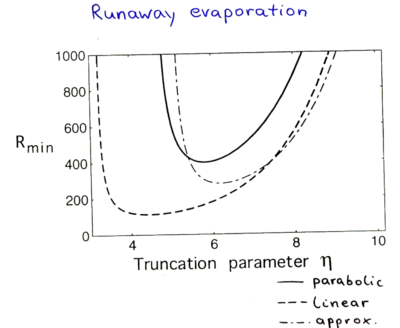
Typical experimental values for are on the order of a few hundred. Since and are functions of , it is clear that is also a function of . It's dependence for a few different trap potentials are plotted below. The dash-dot line is the curve for a parabolic potential using the approximations made here. The other two curves are made using the more accurate Amsterdam model, with the solid line depicting the result for a parabolic potential and the dashed line depicting the result for a linear potential.
When is too large, the cooling proceeds too slowly and atoms are lost to background gas collisions. When is too small, atoms that aren't much warmer than average leave the trap and so the atom number goes down too fast relative to the temperature. That prevents the density from increasing fast enough for runaway evaporation.
Efficiency of Evaporative Cooling
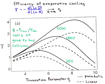
The end goal of an evaporation sequence is to produce a BEC, which requires both low temperatures and high densities. Therefore, to characterize how well evaporation is working, it is not sufficient to simply look at how well one can trade atom number for temperature decreases. A more significant parameter to consider is how the atom number can be traded for increases in phase space density. In the same way we defined as the parameter describing the efficiency of trading fractional atom number decreases for fractional temperature decreases, we can define as the parameter describing the efficiency of trading fractional atom number decreases for fractional phase space density increases.
Below we plot as a function of the truncation parameter for varying values of and for both linear (dashed lines) and parabolic (solid lines) traps. For accuracy the plot is generated with the Amsterdam model. A plot for the results with the approximations made here is available in the references.
Again, the same trade offs between low and high are apparent. However in this metric the parabolic trap outperforms the linear one.
Typical Evaporation Scenario
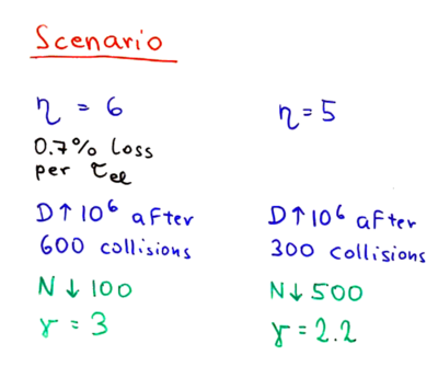
Numbers for typical evaporation scenarios are presented in the graphic below.
With there is an decrease in atom number every elastic collision period. It takes 600 collisions to increase the phase space density by six orders of magnitude, which is a typical amount to go from a cold gas to a BEC. Such an evaporation process causes a factor of 100 decrease in the atom number, which gives the process an efficiency of .
Setting a more aggressive truncation parameter of makes it possible to increase the phase space density by six orders of magnitude after only 300 collisions. However, the price paid is that the atom number drops by a factor of 500 instead of 100 for the other scheme. That extra cost in atom number gives this value of a of only 2.2, less than that of the first scheme.
RF-Induced Evaporation
As discussed above, evaporation requires adjusting the trap depth so that hot atoms may escape. The most obvious way to do this is to ramp down whatever is creating your trap, such as your current for a magnetic trap or laser power for a dipole trap. However, that technique is not ideal because as the trap depth is ramped down, the spring constant that keeps the atoms near the center of the trap is also ramped down. This allows the gas to expand more than it otherwise would, thereby decreasing the cloud density and evaporation rate.
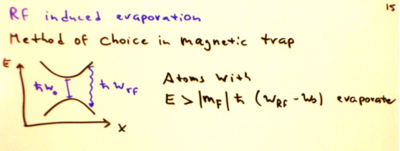
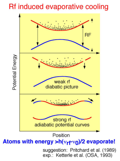
In magnetic traps there is a clever solution for this effect: RF-induced evaporation. It is the method of choice for evaporation in magnetic traps and is conceptually easy to understand. For the simplest model consider an atom with two different magnetic states that are connected via an RF transition. One level should be a trapable low-field seeking state and the other should be an anti-trapped high-field seeking state. Atoms are prepared in the trapable state in loaded into the magnetic trap. An RF field is applied to the atoms which is tuned so that atoms with a large Zeeman shift are on resonance and can be transferred to the anti-trapped state. As a rough approximation we can say that atoms stay near the center of the trap until collisions give an atom enough energy to reach the high-field region. There the RF field transfers the atom to the anti-trapped state and the atom leaves the trap, thus evaporating. Tuning the RF frequency changes where the atoms become resonant with the RF and therefore controls what energy atoms need to leave the trap. In particular, atoms with energy are able to evaporate where is the energy splitting between the two levels at the trap center. Adjusting the RF frequency as the atoms evaporate allows the experimenter to keep fixed without lowering the trap frequency, thus keeping the atomic cloud dense and improving the evaporation.
The above description is a good model in the limit of weak RF drive. An additional detail worth noting is that for weak RF, the atoms do not always transfer to the anti-trapped state and can sometimes fly past the RF resonance region. Therefore a slightly better way to imagine the potential would be as a parabola with a hole cut in it around the RF resonance point, as depicted in the figure below.
For strong RF drive it is more appropriate to analyze the situation in the dressed state basis where the two atomic levels are mixed by the RF. This leads to the curved potential in the bottom of the following figure where the atoms are adiabatically transferred between the two states as they move through the RF resonance region. However, the end result is still the same, the confining potential near the trap center remains strong as the trap depth is ramped down, which would not be the case if the trap depth was lowered by decreasing the current through the magnetic field coils.
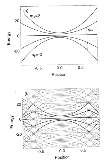
For real alkali atoms the actual level structure is somewhat more complex due to the presence of many Zeeman states. However, the same transition from a trapable state to an anti-trapped state can be performed by transferring through intermediate states. as depicted in the figure below.
Cooling Limits for Evaporative Cooling
Evaporative cooling doesn't involve scattering photons, so it is not affected by the Doppler limit, recoil limit, etc. In fact there is no fundamental limit on the temperatures achievable with evaporative cooling. In practice, technical issues limit the attainable temperatures. Background gas collision rates give a limit on how slowly evaporation can take place, which in turn limits how cold the cloud can get. Additionally, residual heating mechanisms, such as trap vibrations can prevent evaporation from cooling the cloud below an equilibrium temperature. Furthermore, other loss mechanisms, such as three-body loss hamper the performance of evaporation. However, the technique is still sufficient for achieving sub-nanokelvin temperatures. These temperatures are far colder than the cosmic microwave background, which means that these BECs are the coldest known regions in the universe. It's not unlikely that the only colder places are experiments in alien labs on other planets!
References
- Further reading on magnetic trapping: W. K., D.S. Durfee, D.M. Stamper-Kurn, Varenna Lecture Notes 1999, pp. 80-89
- Further reading on evaporative cooling:: W. Ketterle and N.J. van Druten, Adv. At. Mol. Opt. Phys. 37, 181-236 (1986). Relevant pages: pp. 181-193















![{\displaystyle {\dot {N}}=-N{\bigg [}2e^{-\eta }{\sqrt {\frac {\eta }{\pi }}}{\bigg ]}{\bigg [}\sigma n_{0}{\sqrt {\pi \eta }}{\frac {\bar {v}}{2}}{\bigg ]}=-Nn_{0}\sigma {\bar {v}}\eta e^{-\eta }={\frac {-N}{\tau _{ev}}}}](https://wikimedia.org/api/rest_v1/media/math/render/svg/d719d1c2b5558f706eb780f1235945b84d86503a)


![{\displaystyle {\frac {-1}{\lambda \tau _{el}}}={\frac {\dot {N}}{N}}={\frac {{\frac {\mathrm {d} }{\mathrm {d} t}}\left[(n\sigma v)^{\frac {1}{1-\alpha (\delta -1/2)}}\right]}{(n\sigma v)^{\frac {1}{1-\alpha (\delta -1/2)}}}}={\frac {1}{1-\alpha (\delta -1/2)}}{\frac {(n\sigma v)^{{\frac {1}{1-\alpha (\delta -1/2)}}-1}}{(n\sigma v)^{\frac {1}{1-\alpha (\delta -1/2)}}}}{\frac {\mathrm {d} }{\mathrm {d} t}}(n\sigma v)={\frac {1}{1-\alpha (\delta -1/2)}}{\frac {{\frac {\mathrm {d} }{\mathrm {d} t}}(n\sigma v)}{(n\sigma v)}}}](https://wikimedia.org/api/rest_v1/media/math/render/svg/8c59f4cb1d6e6609da013c2a4eaa1c5137f43e34)
![{\displaystyle {\frac {\mathrm {d} (n\sigma v)}{(n\sigma v)}}=-\left[{\frac {1-\alpha (\delta -1/2)}{\lambda }}\right]{\frac {\mathrm {d} t}{\tau _{ev}}}}](https://wikimedia.org/api/rest_v1/media/math/render/svg/bb5ea8e478c18f6781bc98bf19fdaa8522ae0cad)

![{\displaystyle {\frac {\mathrm {d} (n\sigma v)}{(n\sigma v)}}=-\left[{\frac {1-\alpha (\delta -1/2)}{\lambda }}\right]{\frac {\mathrm {d} t}{\tau _{ev}}}-{\frac {\mathrm {d} t}{\tau _{loss}}}=\left[{\frac {\alpha (\delta -1/2)-1}{\lambda }}-{\frac {1}{R}}\right]{\frac {\mathrm {d} t}{\tau _{ev}}}}](https://wikimedia.org/api/rest_v1/media/math/render/svg/8bf699386fdd1be6997ae05f08dfc85ec06b4888)


