Resonances
Contents
- 1 Resonances and Two-Level Atoms
- 1.1 Introduction to Resonances and Precision Measurements
- 1.2 Classical Resonances
- 1.3 Resonance Widths and Uncertainty Relations
- 1.4 Resonances and Two-Level Systems
- 1.5 Quantized Spin in a Magnetic Field
- 1.5.1 Equation of Motion for the Expectation Value
- 1.5.2 The Two-Level System: Spin-\texorpdfstring{Failed to parse (MathML with SVG or PNG fallback (recommended for modern browsers and accessibility tools): Invalid response ("Math extension cannot connect to Restbase.") from server "https://wikimedia.org/api/rest_v1/":): {\displaystyle 1/2} }{1/2}
- 1.5.3 Matrix form of Hamiltonian
- 1.5.4 Solution of the Schrodinger Equation for Spin-\texorpdfstring{Failed to parse (MathML with SVG or PNG fallback (recommended for modern browsers and accessibility tools): Invalid response ("Math extension cannot connect to Restbase.") from server "https://wikimedia.org/api/rest_v1/":): {\displaystyle 1/2} }{1/2} in the Interaction Representation
- 1.5.5 Atomic Clocks and the Ramsey Method
- 1.6 Decoherence Processes, Mixed States, Density Matrix
Resonances and Two-Level Atoms
Introduction to Resonances and Precision Measurements
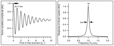
Classically, a resonance is a system where one or more variables change periodically such that when the system is no longer driven by an extended periodic process, the decay of the system's oscillation takes many (or at least several) oscillation periods. Equivalently, the response of the driven system as a function of drive frequency exhibits some form of peaked structure. The frequency corresponding to the maximum response of the system is called the resonance frequency () \begin{figure}
\caption{A resonance in the time (left) and frequency (right) domains. The time domain picture shows the (decaying) oscillation in some variable of the undriven system, while the frequency-domain pictures shows the steady-state response amplitude of the driven system. The time units are chosen such that while the quality factor is .}
\end{figure} The simplest resonance systems have a single resonance frequency, corresponding to the harmonic motion of the variable. Some form of dissipation (damping) results in a finite damping time () for the undriven system, and a finite width () of the resonance curve for the driven system. The quantities and are related by a Fourier transformation: any oscillation with time-varying amplitude must be made up of a superposition of different frequency components, giving the resonance curve a finite width in frequency space. Low dissipation results in a long decay time , and a narrow frequency width . The ratio of frequency width to resonance frequency is called the quality factor .
Atomic physics often deals with isolated atomic systems in a vacuum, providing resonances of high quality factor . For example, an optical transition, even in a room-temperature (ie Doppler-broadened) gas, will have a -factor of
- Failed to parse (unknown function "\unit"): {\displaystyle \frac{f_0}{\Delta f} \sim \frac{\unit{10^{15}}{\hertz}}{\unit{10^9}{\hertz}} \sim 10^6 }
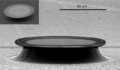
In contrast, high factors in solids typically require cryogenic temperatures: typical factors of mechanical or electrical systems are at room temperature and at Failed to parse (unknown function "\unit"): {\displaystyle \lesssim \unit{1}{\kelvin}} temperatures. Solid optical resonators are an exception to this: has been achieved in the whispering gallery modes of spheres or cylinders of high-purity glass \cite{Armani2003}. \begin{figure}
\caption{One of the whispering-gallery resonators described in \cite{Armani2003}. This particular resonator had a quality factor . The very high surface quality required for such low losses is achieved by having surface tension shape the rim of the disk after it has been temporarily liquefied by a laser pulse; the inset shows the resonator before this treatment.}
\end{figure} At the macroscopic scale, astronomical systems consisting of massive bodies travelling essentially undisturbed through the near-vacuum of space can also exhibit high factors. A resonance is particularly useful for science and technology if it is reproducible by different realizations of the same system, and if it has a well-understood theoretical connection to fundamental constants. In atomic physics, quantum mechanics ensures both features: atoms of the same species are fundamentally identical (although the probing apparatus is not), and the quantum mechanical description of atomic structure is well understood and highly accurate, at least for atoms with not too many electrons. The resonance frequencies of hydrogen, and to a lesser degree helium, are directly tied via quantum mechanics to fundamental constants such as the Rydberg constant, Failed to parse (unknown function "\unit"): {\displaystyle R_\infty=\unit{1.0973731568525(73)\times10^7}{\reciprocal\metre}} \cite{codata2002}, or the fine structure constant \cite{codata2002}. In fact, the Rydberg constant is the most accurately known constant in all of physics, and most fundamental constants have been determined by atomic physics or optical techniques. Additional motivation for measuring fundamental constants with ever-increasing accuracy has been provided by the speculation (and claims of evidence for it \cite{Flambaum2004,Reinhold2006}), that the fundamental constants may not be so constant after all, but that their value is tied to the evolution (and therefore the age) of the universe. Furthermore unexpected resonances, or splittings of resonances, have in the past indicated the need for new theories or modifications of theories. For instance, "anomalous" effects in the Zeeman structure (magnetic-field dependance) of atomic lines led to the discovery of spin \cite{Uhlenbeck1926}. while Lamb's measurement of the splitting between the and states of atomic hydrogen, on the order of \unit{1000}{\mega\hertz} instead of 0 as predicted by the Dirac theory, fostered the development of quantum electrodynamics, the quantum theory of light.
Classical Resonances
A classical harmonic oscillator (HO) is a system described by the second order differential equation
such as a mass on a spring, or a charge, voltage, or currant in an electric RLC resonant circuit. For weak damping () the undriven system decays with an exponential envelope,
with . In the cases we will consider, so that . The decay rate constant for the amplitude is , while for the stored energy it is , i.e. the stored energy decays exponentially with a time constant . If the harmonic oscillator is driven at a frequency close to resonance, , the amplitude response is a lorentzian:
where is the detuning as shown on the right-hand side of Figure \ref{fig:example_resonances}. The full width at half maximum (FWHM) of a lorentzian curve is leading to a quality factor
Note that , , and are measured in angular frequency units \unit{\radian\per\second}, or \unit{\reciprocal\second} for short, and should not be confused with frequencies , etc. When quoting values, we will often write explicitly Failed to parse (unknown function "\unit"): {\displaystyle \omega_0=2\pi\times\unit{1}{\mega\hertz}} rather than Failed to parse (unknown function "\unit"): {\displaystyle \omega_0=\unit{6.28\times10^6}{\reciprocal\second}} to remind ourselves that the quantity in question is an angular frequency. We will never write Failed to parse (unknown function "\unit"): {\displaystyle \omega_0=\unit{6.28\times10^6}{Hz}} : although formally dimensionally consistent, this invites confusion with real (laboratory or Hertzian) frequencies. For brevity, we will often write or say "frequency" when we mean angular frequency, but will quote real frequencies as Failed to parse (unknown function "\unit"): {\displaystyle f_0=\unit{1}{\mega\hertz}} . Note that the natural unit for decay rate constants is that of an angular frequency, as in . Therefore we will express decay rates as inverse times in angular frequency units: Failed to parse (unknown function "\unit"): {\displaystyle \gamma=\unit{10^4}{\reciprocal\second}} for instance, but not Failed to parse (unknown function "\unit"): {\displaystyle \gamma=\unit{10^4}{\hertz}} , nor Failed to parse (unknown function "\unit"): {\displaystyle \gamma=2\pi\times\unit{1.6}{\kilo\hertz}} . Damping time constants are the inverse of decay rate constants, Failed to parse (unknown function "\unit"): {\displaystyle \tau=1/\gamma=\unit{100}{\micro\second}} .
Resonance Widths and Uncertainty Relations
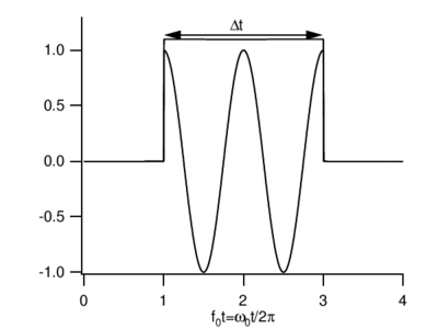
From it follows that damping time and the resonance linewidth of the driven system obey: or, assuming , : a finite number of frequency components or energies () is necessary to synthesize a pulse of finite () width in time. \begin{figure}
\caption{Measurement in a limited time , modelled as an ideal monochromatic sine wave of frequency gated by an observation window of finite width }
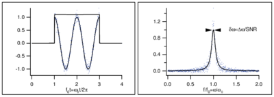
\end{figure} This is quite similar to an uncertainty relation familiar from Fourier transformation theory, according to which the measurement of a frequency in a finite time (see Figure \ref{fig:gated_pulse}) results in a frequency spread obeying . By using we can further connect this with the usual Heisenberg uncertainty relation \QA{ Does the Heisenberg uncertainty relation , or rather the frequency uncertainty relation that follows from (classical) Fourier theory hold in classical systems? Can you measure the angular frequency of a classical harmonic oscillator in a time with an accuracy better than ? }{ Yes: if you have a good model for the signal, for instance if you know that it is a pure sine wave, and if the signal to noise ratio (SNR) of the measurement is good enough, then you can fit the sine wave's frequency to much better accuracy than its spectral width (see Fig. \ref{fig:line_splitting}). As a general rule, the line center can be found to within an uncertainty . This is known as splitting the line. Splitting the line by a factor of 100 is fairly straightforward, splitting it by a factor of a 1000 is a real challenge. As an extreme example of this, Caesium fountain clocks interrogate a \unit{9}{\giga\hertz} transition for a typical measurement time of \unit{1}{\second}, yielding , but the best ones can nonetheless achieve relative accuracies of \cite{Santarelli1999}. Of course, this sort of performance requires a very good understanding of the line shape and of systematics. } \begin{figure}
\caption{Splitting the line in time and frequency domains. Given a sufficiently good model of the signal or line shape, and adequate signal-to-noise, one can find the center frequency of the underlying signal to much better than or the line width.}
\end{figure} \QU{ Can you measure the angular frequency of a quantum mechanical harmonic oscillator in a time to better than ? } \QU{ Can you measure the angular frequency of a laser pulse lasting a time to better than ?} If you answered \ref{q:quantum_line_splitting} and \ref{q:classical_line_splitting} differently, you may have a problem with \ref{q:laser_line_splitting}. Is a laser pulse quantum or classical? Clearly it is possible to beat for a laser pulse. For instance, you can superimpose the laser pulse with a laser of fixed and known frequency on a photodiode, and fit the observed beatnote. The stronger the probe pulse, the better the SNR of the beatnote, and the more accurately you can extract the probe frequency. So how are we to reconcile quantum mechanics and classical mechanics, and what does the Heisenberg uncertainty really state? The Heisenberg uncertainty relation makes a statement about predicting the outcome of a single measurement on a single system. For a single photon, the limit does indeed hold. However, nothing in quantum mechanics says that you cannot improve your knowledge about the average values of the quantities characterizing the system by repeated measurements on identical copies of it. In the laser example above, the frequency resolution improves with probe pulse strength because we are measuring many photons - for the purposes of this discussion we could have measured the frequencies of the photons sequentially. For independent measurement of uncorrelated photons the SNR is given by : the signal grows as , while the noise is the shot noise of the photon number, which grows as . This SNR allows a frequency uncertainty of , known as the standard quantum limit. If we allow the use of entangled or correlated states of the photons, then the uncertainty can be as low as the Heisenberg limit \cite{Wineland1992,Wineland1994}. Let us now revisit \ref{q:quantum_line_splitting}. You may have heard that the quantum mechanical description of electromagnetism, quantum electrodynamics (QED), represents any single mode of the electromagnetic field by a harmonic oscillator of the same frequency. The ground state corresponds to no photons in the mode, the first excited state to one photon and so forth. This description is valid because photons to a very good approximation do not interact: the addition of a photon changes the system's energy always by the same increment. Since the many-photon pulse from \ref{q:laser_line_splitting} maps onto a quantum harmonic oscillator, it seems to follow that \ref{q:quantum_line_splitting} must also be answered in the affirmative. On the other hand, a harmonic oscillator is a single quantum system to which the Heisenberg limit must apply. The resolution of this apparent contradiction is that \ref{q:quantum_line_splitting} is asking about a measurement of the fundamental frequency of the harmonic oscillator, not the energy of a particular level. Therefore if you measure the energy of the n-th level to , which can be done by exciting the -th level from the ground state through a nonlinear process, then the uncertainty on the harmonic oscillator resonance frequency (that corresponds to the laser frequency in \ref{q:quantum_line_splitting}) is given by . �If the interaction with the oscillator is restricted to classical fields or forces, then there is an additional uncertainty of on which particular level of the oscillator is being measured and so we recover the standard quantum limit mentioned previously.
Resonances and Two-Level Systems
Resonances and Two-Level Systems
Quantized Spin in a Magnetic Field
Equation of Motion for the Expectation Value
For the system we have been considering, the Hamiltonian is
Recalling the Heisenberg equation of motion for any operator is
where the last term refers to operators with an explicit time dependence, we have in this instance
Using with the Levi-Civita symbol , we have
or in short
- Failed to parse (MathML with SVG or PNG fallback (recommended for modern browsers and accessibility tools): Invalid response ("Math extension cannot connect to Restbase.") from server "https://wikimedia.org/api/rest_v1/":): {\displaystyle \begin{align} \frac{d}{dt} {\bf{\hat\mu}} &= \gamma {\bf{\hat\mu}} \times {\bf{B}} \\ \frac{d}{dt} {\bf{\hat L}} &= \gamma {\bf{\hat L}} \times {\bf{B}} \end{align}}
These are just like the classical equations of motion \ref{eq:classical_precession_in_static_field}, but here they describe the precession of the operator for the magnetic moment Failed to parse (MathML with SVG or PNG fallback (recommended for modern browsers and accessibility tools): Invalid response ("Math extension cannot connect to Restbase.") from server "https://wikimedia.org/api/rest_v1/":): {\displaystyle {\bf{\hat\mu}} } or for the angular momentum Failed to parse (MathML with SVG or PNG fallback (recommended for modern browsers and accessibility tools): Invalid response ("Math extension cannot connect to Restbase.") from server "https://wikimedia.org/api/rest_v1/":): {\displaystyle {\bf{\hat L}} } about the magnetic field at the (Larmor) angular frequency Failed to parse (MathML with SVG or PNG fallback (recommended for modern browsers and accessibility tools): Invalid response ("Math extension cannot connect to Restbase.") from server "https://wikimedia.org/api/rest_v1/":): {\displaystyle \omega_L=\gamma B_0} . Note that \begin{itemize} \item Just as in the classical model, these operator equations are exact; we have not neglected any higher order terms. \item Since the equations of motion hold for the operator, they must hold for the expectation value
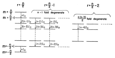
\item We have not made use of any special relations for a spin-Failed to parse (MathML with SVG or PNG fallback (recommended for modern browsers and accessibility tools): Invalid response ("Math extension cannot connect to Restbase.") from server "https://wikimedia.org/api/rest_v1/":): {\displaystyle 1/2} system, but just the general commutation relation for angular momentum. Therefore the result, precession about the magnetic field at the Larmor frequency, remains true for any value of angular momentum Failed to parse (MathML with SVG or PNG fallback (recommended for modern browsers and accessibility tools): Invalid response ("Math extension cannot connect to Restbase.") from server "https://wikimedia.org/api/rest_v1/":): {\displaystyle l} . \item A spin-Failed to parse (MathML with SVG or PNG fallback (recommended for modern browsers and accessibility tools): Invalid response ("Math extension cannot connect to Restbase.") from server "https://wikimedia.org/api/rest_v1/":): {\displaystyle 1/2} system has two energy levels, and the two-level problem with coupling between two levels can be mapped onto the problem for a spin in a magnetic field, for which we have developed a good classical intuition. \item If coupling between two or more angular momenta or spins within an atom results in an angular momentum Failed to parse (MathML with SVG or PNG fallback (recommended for modern browsers and accessibility tools): Invalid response ("Math extension cannot connect to Restbase.") from server "https://wikimedia.org/api/rest_v1/":): {\displaystyle F>1/2} , the time evolution of this angular momentum in an external field is governed by the same physics as for the two-level system. This is true as long as the applied magnetic field is not large enough to break the coupling between the angular momenta; a situation known as the Zeeman regime. Note that if the coupled angular momenta have different gyromagnetic ratios, the gyromagnetic ratio for the composite angular momentum is different from those of the constituents. \item For large magnetic field the interaction of the individual constituents with the magnetic field dominates, and they precess separately about the magnetic field. This is the Paschen-Back regime. \item An even more interesting composite angular momentum arises when two-level atoms are coupled symmetrically to an external field. In this case we have an effective angular momentum Failed to parse (MathML with SVG or PNG fallback (recommended for modern browsers and accessibility tools): Invalid response ("Math extension cannot connect to Restbase.") from server "https://wikimedia.org/api/rest_v1/":): {\displaystyle L=N/2} for the symmetric coupling (see Figure \ref{fig:dicke_states}). \begin{figure}
\caption{Level structure diagram for Failed to parse (MathML with SVG or PNG fallback (recommended for modern browsers and accessibility tools): Invalid response ("Math extension cannot connect to Restbase.") from server "https://wikimedia.org/api/rest_v1/":): {\displaystyle n} two-level atoms in a basis of symmetric states \cite{Dicke1954}. The leftmost column corresponds to an effective spin-Failed to parse (MathML with SVG or PNG fallback (recommended for modern browsers and accessibility tools): Invalid response ("Math extension cannot connect to Restbase.") from server "https://wikimedia.org/api/rest_v1/":): {\displaystyle n/2} object. Other columns correspond to manifolds of symmetric states of the Failed to parse (MathML with SVG or PNG fallback (recommended for modern browsers and accessibility tools): Invalid response ("Math extension cannot connect to Restbase.") from server "https://wikimedia.org/api/rest_v1/":): {\displaystyle n} atoms with lower total effective angular momentum.}
\end{figure} Again the equation of motion for the composite angular momentum is a precession. This is the problem considered in Dicke's famous paper \cite{Dicke1954}, in which he shows that this collective precession can give rise to massively enhanced couplings to external fields ("superradiance") due to constructive interference between the individual atoms. \end{itemize}
The Two-Level System: Spin-\texorpdfstring{Failed to parse (MathML with SVG or PNG fallback (recommended for modern browsers and accessibility tools): Invalid response ("Math extension cannot connect to Restbase.") from server "https://wikimedia.org/api/rest_v1/":): {\displaystyle 1/2} }{1/2}
Let us now specialize to the two-level system and calculate the time evolution of the occupation probabilities for the two levels. \begin{figure}
\caption{Equivalence of two-level system with spin-Failed to parse (MathML with SVG or PNG fallback (recommended for modern browsers and accessibility tools): Invalid response ("Math extension cannot connect to Restbase.") from server "https://wikimedia.org/api/rest_v1/":): {\displaystyle 1/2} . Note that for Failed to parse (MathML with SVG or PNG fallback (recommended for modern browsers and accessibility tools): Invalid response ("Math extension cannot connect to Restbase.") from server "https://wikimedia.org/api/rest_v1/":): {\displaystyle \gamma>0} the spin-up state (spin aligned with field) is the ground state. For an electron, with Failed to parse (MathML with SVG or PNG fallback (recommended for modern browsers and accessibility tools): Invalid response ("Math extension cannot connect to Restbase.") from server "https://wikimedia.org/api/rest_v1/":): {\displaystyle \gamma<0} , spin-up is the excited state. Be careful, as both conventions are used in the literature.}
\end{figure} We have that
where in the last equation we have used the fact that Failed to parse (MathML with SVG or PNG fallback (recommended for modern browsers and accessibility tools): Invalid response ("Math extension cannot connect to Restbase.") from server "https://wikimedia.org/api/rest_v1/":): {\displaystyle P_e+P_g=1} . The signs are chosen for a spin with Failed to parse (MathML with SVG or PNG fallback (recommended for modern browsers and accessibility tools): Invalid response ("Math extension cannot connect to Restbase.") from server "https://wikimedia.org/api/rest_v1/":): {\displaystyle \gamma>0} , such as a proton (Figure \ref{fig:two_level_spin_half}). For an electron, or any other spin with Failed to parse (MathML with SVG or PNG fallback (recommended for modern browsers and accessibility tools): Invalid response ("Math extension cannot connect to Restbase.") from server "https://wikimedia.org/api/rest_v1/":): {\displaystyle \gamma<0} , the analysis would be the same but for the opposite sign of Failed to parse (MathML with SVG or PNG fallback (recommended for modern browsers and accessibility tools): Invalid response ("Math extension cannot connect to Restbase.") from server "https://wikimedia.org/api/rest_v1/":): {\displaystyle S_z} and the corresponding exchange of and Failed to parse (MathML with SVG or PNG fallback (recommended for modern browsers and accessibility tools): Invalid response ("Math extension cannot connect to Restbase.") from server "https://wikimedia.org/api/rest_v1/":): {\displaystyle \downarrow} . If the system is initially in the ground state, Failed to parse (MathML with SVG or PNG fallback (recommended for modern browsers and accessibility tools): Invalid response ("Math extension cannot connect to Restbase.") from server "https://wikimedia.org/api/rest_v1/":): {\displaystyle P_g(t=0)=1} (or the spin along Failed to parse (MathML with SVG or PNG fallback (recommended for modern browsers and accessibility tools): Invalid response ("Math extension cannot connect to Restbase.") from server "https://wikimedia.org/api/rest_v1/":): {\displaystyle + {\bf{\hat e}} _z} , Failed to parse (MathML with SVG or PNG fallback (recommended for modern browsers and accessibility tools): Invalid response ("Math extension cannot connect to Restbase.") from server "https://wikimedia.org/api/rest_v1/":): {\displaystyle S_z(0)=+\hbar/2} ), the expectation value obeys the classical equation of motion \ref{eq:classical_rabi_flopping}:
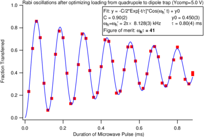
Equation \ref{eqn:rabi_transition_probability} is the probability to find system in the excited state at time Failed to parse (MathML with SVG or PNG fallback (recommended for modern browsers and accessibility tools): Invalid response ("Math extension cannot connect to Restbase.") from server "https://wikimedia.org/api/rest_v1/":): {\displaystyle t} if it was in ground state at time Failed to parse (MathML with SVG or PNG fallback (recommended for modern browsers and accessibility tools): Invalid response ("Math extension cannot connect to Restbase.") from server "https://wikimedia.org/api/rest_v1/":): {\displaystyle t=0} . Figure \ref{fig:rabi_signal} shows a real-world example of such an oscillation. \begin{figure}
\caption{Rabi oscillation signal taken in the Vuleti\'{c} lab shortly after this topic was covered in lecture in 2008. The amplitude of the oscillations decays with time due to spatial variations in the strength of the drive field (and hence of the Rabi frequency), so that the different atoms drift out of phase with each other.}
\end{figure}
Matrix form of Hamiltonian
With the matrix representation
- Failed to parse (MathML with SVG or PNG fallback (recommended for modern browsers and accessibility tools): Invalid response ("Math extension cannot connect to Restbase.") from server "https://wikimedia.org/api/rest_v1/":): {\displaystyle \begin{align} \left|e\right\rangle &= \left|S_z = - \frac{1}{2}\right\rangle = \begin{pmatrix} 1 \\ 0 \end{pmatrix} \\ \left|g\right\rangle &= \left|S_z = + \frac{1}{2}\right\rangle = \begin{pmatrix} 0 \\ 1 \end{pmatrix} \end{align}}
we can write the Hamiltonian Failed to parse (MathML with SVG or PNG fallback (recommended for modern browsers and accessibility tools): Invalid response ("Math extension cannot connect to Restbase.") from server "https://wikimedia.org/api/rest_v1/":): {\displaystyle H_0} associated with the static field as
- Failed to parse (MathML with SVG or PNG fallback (recommended for modern browsers and accessibility tools): Invalid response ("Math extension cannot connect to Restbase.") from server "https://wikimedia.org/api/rest_v1/":): {\displaystyle \hat{H}_0 = - {\bf{\hat\mu}} \cdot {\bf{B}} _0 = - \gamma \hat{S}_z B_0 = - \hbar \omega_0 \frac{\hat{S}_z}{\hbar} = \frac{1}{2} \hbar \omega_0 \begin{pmatrix} 1 & 0 \\ 0 & -1 \end{pmatrix} = \frac{1}{2} \hbar \omega_0 \hat{\sigma}_z }
where Failed to parse (MathML with SVG or PNG fallback (recommended for modern browsers and accessibility tools): Invalid response ("Math extension cannot connect to Restbase.") from server "https://wikimedia.org/api/rest_v1/":): {\displaystyle \omega_0=\gamma B_0} is the Larmor frequency, and
- Failed to parse (MathML with SVG or PNG fallback (recommended for modern browsers and accessibility tools): Invalid response ("Math extension cannot connect to Restbase.") from server "https://wikimedia.org/api/rest_v1/":): {\displaystyle \hat{\sigma}_z= \begin{pmatrix} 1 & 0 \\ 0 & -1 \end{pmatrix} }
is a Pauli spin matrix. The eigenstates are Failed to parse (MathML with SVG or PNG fallback (recommended for modern browsers and accessibility tools): Invalid response ("Math extension cannot connect to Restbase.") from server "https://wikimedia.org/api/rest_v1/":): {\displaystyle \left|e\right\rangle } , with eigenenergies . A spin initially along , corresponding to
evolves in time as
- Failed to parse (MathML with SVG or PNG fallback (recommended for modern browsers and accessibility tools): Invalid response ("Math extension cannot connect to Restbase.") from server "https://wikimedia.org/api/rest_v1/":): {\displaystyle \left|\psi(t)\right\rangle =\frac{1}{\sqrt{2}} \left(e^{-i\omega_0 t / 2} \left|e\right\rangle +e^{+i\omega_0 t / 2} \left|g\right\rangle \right) =\frac{e^{-i\omega_0 t/2}}{\sqrt{2}}\left( \left|e\right\rangle +e^{i\omega_0 t} \left|g\right\rangle \right) }
which describes a precession with angluar frequency Failed to parse (MathML with SVG or PNG fallback (recommended for modern browsers and accessibility tools): Invalid response ("Math extension cannot connect to Restbase.") from server "https://wikimedia.org/api/rest_v1/":): {\displaystyle \omega_0} . The field Failed to parse (MathML with SVG or PNG fallback (recommended for modern browsers and accessibility tools): Invalid response ("Math extension cannot connect to Restbase.") from server "https://wikimedia.org/api/rest_v1/":): {\displaystyle {\bf{B}} _1} , rotating at Failed to parse (MathML with SVG or PNG fallback (recommended for modern browsers and accessibility tools): Invalid response ("Math extension cannot connect to Restbase.") from server "https://wikimedia.org/api/rest_v1/":): {\displaystyle \omega} in the plane corresponds to
- Failed to parse (MathML with SVG or PNG fallback (recommended for modern browsers and accessibility tools): Invalid response ("Math extension cannot connect to Restbase.") from server "https://wikimedia.org/api/rest_v1/":): {\displaystyle \begin{align} \hat{H}_1 &= - {\bf{\hat\mu}} \cdot {\bf{B}} _1(t) =- {\bf{\hat\mu}} \cdot\frac{\omega_R}{\gamma} \left(- {\bf{\hat e}} _x \cos\omega t- {\bf{\hat e}} _y \sin\omega t\right) \\ &= \omega_R\left(\hat{S}_x \cos\omega t + \hat{S}_y \sin\omega t\right) \\ &= \frac{\hbar\omega_R}{2} \left(\hat{\sigma}_x \cos\omega t + \hat{\sigma}_y \sin\omega t\right) \\ &= \frac{\hbar\omega_R}{2} \left( \begin{pmatrix} 0 & 1 \\ 1 & 0 \end{pmatrix}\cos\omega t + \begin{pmatrix} 0 & -i \\ i & 0 \end{pmatrix}\sin\omega t \right) \\ \hat{H}_1 &= \frac{\hbar\omega_R}{2} \begin{pmatrix} 0 & e^{-i\omega t} \\ e^{i\omega t} & 0 \end{pmatrix} \end{align}}
where have used the Pauli spin matrices Failed to parse (MathML with SVG or PNG fallback (recommended for modern browsers and accessibility tools): Invalid response ("Math extension cannot connect to Restbase.") from server "https://wikimedia.org/api/rest_v1/":): {\displaystyle \sigma_x} , Failed to parse (MathML with SVG or PNG fallback (recommended for modern browsers and accessibility tools): Invalid response ("Math extension cannot connect to Restbase.") from server "https://wikimedia.org/api/rest_v1/":): {\displaystyle \sigma_y} . The full Hamiltonian is thus given by
- Failed to parse (MathML with SVG or PNG fallback (recommended for modern browsers and accessibility tools): Invalid response ("Math extension cannot connect to Restbase.") from server "https://wikimedia.org/api/rest_v1/":): {\displaystyle \hat{H}=\frac{\hbar}{2} \begin{pmatrix} +\omega_0 & \omega_R e^{-i \omega t} \\ \omega_R e^{-i \omega t} & - \omega_0 \end{pmatrix} }
This is the famous "dressed atom" Hamiltonian in the so-called "rotating wave approximation". Its eigenstates and eigenvalues provide a very elegant, very intuitive solution to the two-state problem.
Solution of the Schrodinger Equation for Spin-\texorpdfstring{Failed to parse (MathML with SVG or PNG fallback (recommended for modern browsers and accessibility tools): Invalid response ("Math extension cannot connect to Restbase.") from server "https://wikimedia.org/api/rest_v1/":): {\displaystyle 1/2} }{1/2} in the Interaction Representation
The interaction representation consists of expanding the state Failed to parse (MathML with SVG or PNG fallback (recommended for modern browsers and accessibility tools): Invalid response ("Math extension cannot connect to Restbase.") from server "https://wikimedia.org/api/rest_v1/":): {\displaystyle \left|\psi(t)\right\rangle } in terms of the eigenstates Failed to parse (MathML with SVG or PNG fallback (recommended for modern browsers and accessibility tools): Invalid response ("Math extension cannot connect to Restbase.") from server "https://wikimedia.org/api/rest_v1/":): {\displaystyle \left|e\right\rangle } , Failed to parse (MathML with SVG or PNG fallback (recommended for modern browsers and accessibility tools): Invalid response ("Math extension cannot connect to Restbase.") from server "https://wikimedia.org/api/rest_v1/":): {\displaystyle \left|g\right\rangle } of the Hamiltonian Failed to parse (MathML with SVG or PNG fallback (recommended for modern browsers and accessibility tools): Invalid response ("Math extension cannot connect to Restbase.") from server "https://wikimedia.org/api/rest_v1/":): {\displaystyle H_0} , including their known time dependence Failed to parse (MathML with SVG or PNG fallback (recommended for modern browsers and accessibility tools): Invalid response ("Math extension cannot connect to Restbase.") from server "https://wikimedia.org/api/rest_v1/":): {\displaystyle e^{iH_0 t/\hbar}} due to Failed to parse (MathML with SVG or PNG fallback (recommended for modern browsers and accessibility tools): Invalid response ("Math extension cannot connect to Restbase.") from server "https://wikimedia.org/api/rest_v1/":): {\displaystyle H_0} . That means we write here
- Failed to parse (MathML with SVG or PNG fallback (recommended for modern browsers and accessibility tools): Invalid response ("Math extension cannot connect to Restbase.") from server "https://wikimedia.org/api/rest_v1/":): {\displaystyle \left|\psi(t)\right\rangle =a_e(t) \left|e\right\rangle e^{-i\omega_0t/2}+a_g(t) \left|g\right\rangle e^{i\omega_0t/2} }
Substituting this into the Schrodinger equation
- Failed to parse (MathML with SVG or PNG fallback (recommended for modern browsers and accessibility tools): Invalid response ("Math extension cannot connect to Restbase.") from server "https://wikimedia.org/api/rest_v1/":): {\displaystyle i\hbar\frac{d}{dt} \left|\psi(t)\right\rangle =\left(H_0+H_1\right) \left|\psi(t)\right\rangle }
then results in the equations of motion for the coefficients
- Failed to parse (MathML with SVG or PNG fallback (recommended for modern browsers and accessibility tools): Invalid response ("Math extension cannot connect to Restbase.") from server "https://wikimedia.org/api/rest_v1/":): {\displaystyle \begin{align} i\dot{a}_e&= \frac{\omega_R}{2}e^{i\left(\omega_0-\omega\right)t}a_g \\ i\dot{a}_g&= \frac{\omega_R}{2}e^{-i\left(\omega_0-\omega\right)t}a_e \end{align}}
Where we have used the matrix form of the Hamiltonian, \ref{eq:dressed_atom_hamiltonian}. Introducing the detuning Failed to parse (MathML with SVG or PNG fallback (recommended for modern browsers and accessibility tools): Invalid response ("Math extension cannot connect to Restbase.") from server "https://wikimedia.org/api/rest_v1/":): {\displaystyle \delta=\omega-\omega_0} , we have
- Failed to parse (MathML with SVG or PNG fallback (recommended for modern browsers and accessibility tools): Invalid response ("Math extension cannot connect to Restbase.") from server "https://wikimedia.org/api/rest_v1/":): {\displaystyle \begin{align} i\dot{a}_g&= \frac{\omega_R}{2}e^{i\delta t}a_e \\ i\dot{a}_e&= \frac{\omega_R}{2}e^{-i\delta t}a_g \end{align}}
The explicit time dependence can be eliminated by the sustitution
- Failed to parse (MathML with SVG or PNG fallback (recommended for modern browsers and accessibility tools): Invalid response ("Math extension cannot connect to Restbase.") from server "https://wikimedia.org/api/rest_v1/":): {\displaystyle \begin{align} b_g&= e^{-i\delta t/2}a_g \\ b_e&= e^{i\delta t/2}a_e \end{align}}
As you will show (or have shown) in the problem set, this leads to solutions for Failed to parse (MathML with SVG or PNG fallback (recommended for modern browsers and accessibility tools): Invalid response ("Math extension cannot connect to Restbase.") from server "https://wikimedia.org/api/rest_v1/":): {\displaystyle b_{g,e}} given by
- Failed to parse (MathML with SVG or PNG fallback (recommended for modern browsers and accessibility tools): Invalid response ("Math extension cannot connect to Restbase.") from server "https://wikimedia.org/api/rest_v1/":): {\displaystyle \begin{align} b_g(t)&= e^{i\Omega_R t/2}B_1+e^{-i\Omega_R t/2}B_2 \\ b_e(t)&= \frac{\omega_R}{\delta-\Omega_R}e^{i\Omega t/2}B_1 +\frac{\omega_R}{\delta+\Omega_R}e^{-i\Omega_R t/2}B_2 \end{align}}
with two constants that are determined by the initial conditions. For Failed to parse (MathML with SVG or PNG fallback (recommended for modern browsers and accessibility tools): Invalid response ("Math extension cannot connect to Restbase.") from server "https://wikimedia.org/api/rest_v1/":): {\displaystyle a_g(t=0)=1} we find
- Failed to parse (MathML with SVG or PNG fallback (recommended for modern browsers and accessibility tools): Invalid response ("Math extension cannot connect to Restbase.") from server "https://wikimedia.org/api/rest_v1/":): {\displaystyle \left| a_e(t)\right| ^2=\frac{\omega_R^2}{\Omega_R^2}\sin^2\frac{\Omega_R t}{2} }
as already derived from the fact that the expectation value for the magnetic moment obeys the classical equation.
Atomic Clocks and the Ramsey Method
When comparing the Hamiltonian for a spin-Failed to parse (MathML with SVG or PNG fallback (recommended for modern browsers and accessibility tools): Invalid response ("Math extension cannot connect to Restbase.") from server "https://wikimedia.org/api/rest_v1/":): {\displaystyle 1/2} in a magnetic field to that of a two-level system with a coupling between the two levels characterized by the strength Failed to parse (MathML with SVG or PNG fallback (recommended for modern browsers and accessibility tools): Invalid response ("Math extension cannot connect to Restbase.") from server "https://wikimedia.org/api/rest_v1/":): {\displaystyle \omega_R} and frequency Failed to parse (MathML with SVG or PNG fallback (recommended for modern browsers and accessibility tools): Invalid response ("Math extension cannot connect to Restbase.") from server "https://wikimedia.org/api/rest_v1/":): {\displaystyle \omega} , we see that the energy spacing between Failed to parse (MathML with SVG or PNG fallback (recommended for modern browsers and accessibility tools): Invalid response ("Math extension cannot connect to Restbase.") from server "https://wikimedia.org/api/rest_v1/":): {\displaystyle \left|e\right\rangle } and Failed to parse (MathML with SVG or PNG fallback (recommended for modern browsers and accessibility tools): Invalid response ("Math extension cannot connect to Restbase.") from server "https://wikimedia.org/api/rest_v1/":): {\displaystyle \left|g\right\rangle } corresponds to the Larmor frequency Failed to parse (MathML with SVG or PNG fallback (recommended for modern browsers and accessibility tools): Invalid response ("Math extension cannot connect to Restbase.") from server "https://wikimedia.org/api/rest_v1/":): {\displaystyle \omega_0} in the static field. This spacing can provide a frequency or time reference if perturbations affecting Failed to parse (MathML with SVG or PNG fallback (recommended for modern browsers and accessibility tools): Invalid response ("Math extension cannot connect to Restbase.") from server "https://wikimedia.org/api/rest_v1/":): {\displaystyle \omega_0} are sufficiently well controlled. For instance, the time unit "second" is defined via the transition frequency between two hyperfine states in the electronic ground state of the caesium atom, which is near \unit{9.2}{\giga\hertz} in the microwave domain. The task of an atomic clock is then to measure this frequency accurately by trying to tune a frequency source (the frequency of the rotating field Failed to parse (MathML with SVG or PNG fallback (recommended for modern browsers and accessibility tools): Invalid response ("Math extension cannot connect to Restbase.") from server "https://wikimedia.org/api/rest_v1/":): {\displaystyle B_1} in the spin picture) to the atomic frequency Failed to parse (MathML with SVG or PNG fallback (recommended for modern browsers and accessibility tools): Invalid response ("Math extension cannot connect to Restbase.") from server "https://wikimedia.org/api/rest_v1/":): {\displaystyle \omega_0} . Equivalently, we want to find the frequency Failed to parse (MathML with SVG or PNG fallback (recommended for modern browsers and accessibility tools): Invalid response ("Math extension cannot connect to Restbase.") from server "https://wikimedia.org/api/rest_v1/":): {\displaystyle \omega} such that the detuning Failed to parse (MathML with SVG or PNG fallback (recommended for modern browsers and accessibility tools): Invalid response ("Math extension cannot connect to Restbase.") from server "https://wikimedia.org/api/rest_v1/":): {\displaystyle \delta=\omega-\omega_0} is equal to zero. Starting with an atom in (spin along Failed to parse (MathML with SVG or PNG fallback (recommended for modern browsers and accessibility tools): Invalid response ("Math extension cannot connect to Restbase.") from server "https://wikimedia.org/api/rest_v1/":): {\displaystyle + {\bf{\hat e}} _z} for Failed to parse (MathML with SVG or PNG fallback (recommended for modern browsers and accessibility tools): Invalid response ("Math extension cannot connect to Restbase.") from server "https://wikimedia.org/api/rest_v1/":): {\displaystyle \gamma>0} ), we could try to find the resonance frequency by noting that according to
- Failed to parse (MathML with SVG or PNG fallback (recommended for modern browsers and accessibility tools): Invalid response ("Math extension cannot connect to Restbase.") from server "https://wikimedia.org/api/rest_v1/":): {\displaystyle P_e(t)=\frac{\omega_R^2}{\omega_R^2+\delta^2} sin^2\left(\sqrt{\omega_R^2+\delta^2}\,\frac{t}{2}\right) }
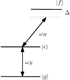
the population of the upper state is maximized for Failed to parse (MathML with SVG or PNG fallback (recommended for modern browsers and accessibility tools): Invalid response ("Math extension cannot connect to Restbase.") from server "https://wikimedia.org/api/rest_v1/":): {\displaystyle \delta=0} (i.e. the precession of the spin to the direction is only complete on resonance). This is the so-called Rabi method. It suffers from a number of drawbacks. For one, the signal is only quadratic in the detuning Failed to parse (MathML with SVG or PNG fallback (recommended for modern browsers and accessibility tools): Invalid response ("Math extension cannot connect to Restbase.") from server "https://wikimedia.org/api/rest_v1/":): {\displaystyle \delta} , i.e. the method is relatively insensitive near Failed to parse (MathML with SVG or PNG fallback (recommended for modern browsers and accessibility tools): Invalid response ("Math extension cannot connect to Restbase.") from server "https://wikimedia.org/api/rest_v1/":): {\displaystyle \delta=0} . Furthermore, the optimum time Failed to parse (MathML with SVG or PNG fallback (recommended for modern browsers and accessibility tools): Invalid response ("Math extension cannot connect to Restbase.") from server "https://wikimedia.org/api/rest_v1/":): {\displaystyle t} depends on the strength of the coupling (i.e. the strength of the rotating field), so fluctuations in Failed to parse (MathML with SVG or PNG fallback (recommended for modern browsers and accessibility tools): Invalid response ("Math extension cannot connect to Restbase.") from server "https://wikimedia.org/api/rest_v1/":): {\displaystyle \omega_R} can be mistaken for changes in Failed to parse (MathML with SVG or PNG fallback (recommended for modern browsers and accessibility tools): Invalid response ("Math extension cannot connect to Restbase.") from server "https://wikimedia.org/api/rest_v1/":): {\displaystyle \delta} . Finally the coupling by Failed to parse (MathML with SVG or PNG fallback (recommended for modern browsers and accessibility tools): Invalid response ("Math extension cannot connect to Restbase.") from server "https://wikimedia.org/api/rest_v1/":): {\displaystyle \omega_R} to other levels can lead to level shifts that are not intrinsic to the atom, but depend on the applied drive (Figure \ref{fig:rabi_third_level}). \begin{figure}
\caption{The drive used for Rabi flopping within the Failed to parse (MathML with SVG or PNG fallback (recommended for modern browsers and accessibility tools): Invalid response ("Math extension cannot connect to Restbase.") from server "https://wikimedia.org/api/rest_v1/":): {\displaystyle \left|e\right\rangle} , Failed to parse (MathML with SVG or PNG fallback (recommended for modern browsers and accessibility tools): Invalid response ("Math extension cannot connect to Restbase.") from server "https://wikimedia.org/api/rest_v1/":): {\displaystyle \left|g\right\rangle} system can also off-resonantly couple one or both levels to other states, perturbing the transition frequency Failed to parse (MathML with SVG or PNG fallback (recommended for modern browsers and accessibility tools): Invalid response ("Math extension cannot connect to Restbase.") from server "https://wikimedia.org/api/rest_v1/":): {\displaystyle \omega_0} .}
\end{figure} Norman Ramsey invented an alternative method (the so-called "separated oscillatory fields method", known for short as the "Ramsey method" \cite{Ramsey1949,Ramsey1950}, for which he received the Nobel prize), that fixes all of these problems. It leads to a signal that is linear rather than quadratic in the detuning Failed to parse (MathML with SVG or PNG fallback (recommended for modern browsers and accessibility tools): Invalid response ("Math extension cannot connect to Restbase.") from server "https://wikimedia.org/api/rest_v1/":): {\displaystyle \delta} , does not require tuning the measurement time to match the applied field strength Failed to parse (MathML with SVG or PNG fallback (recommended for modern browsers and accessibility tools): Invalid response ("Math extension cannot connect to Restbase.") from server "https://wikimedia.org/api/rest_v1/":): {\displaystyle \omega_R=\gamma B_1} , and, most importantly, eliminates level shifts due to altogether. The method is as follows. Instead of applying a pulse for a time t that corresponds to Rabi rotation of the spin by Failed to parse (MathML with SVG or PNG fallback (recommended for modern browsers and accessibility tools): Invalid response ("Math extension cannot connect to Restbase.") from server "https://wikimedia.org/api/rest_v1/":): {\displaystyle \pi} (called a Failed to parse (MathML with SVG or PNG fallback (recommended for modern browsers and accessibility tools): Invalid response ("Math extension cannot connect to Restbase.") from server "https://wikimedia.org/api/rest_v1/":): {\displaystyle \pi} pulse), the pulse is applied for half that time, corresponding to the Rabi rotation of the spin by Failed to parse (MathML with SVG or PNG fallback (recommended for modern browsers and accessibility tools): Invalid response ("Math extension cannot connect to Restbase.") from server "https://wikimedia.org/api/rest_v1/":): {\displaystyle \pi/2} into the Failed to parse (MathML with SVG or PNG fallback (recommended for modern browsers and accessibility tools): Invalid response ("Math extension cannot connect to Restbase.") from server "https://wikimedia.org/api/rest_v1/":): {\displaystyle X-Y} plane (Failed to parse (MathML with SVG or PNG fallback (recommended for modern browsers and accessibility tools): Invalid response ("Math extension cannot connect to Restbase.") from server "https://wikimedia.org/api/rest_v1/":): {\displaystyle \pi/2} pulse). Then the applied field Failed to parse (MathML with SVG or PNG fallback (recommended for modern browsers and accessibility tools): Invalid response ("Math extension cannot connect to Restbase.") from server "https://wikimedia.org/api/rest_v1/":): {\displaystyle B_1} is turned off and the system is left to precess in the static field Failed to parse (MathML with SVG or PNG fallback (recommended for modern browsers and accessibility tools): Invalid response ("Math extension cannot connect to Restbase.") from server "https://wikimedia.org/api/rest_v1/":): {\displaystyle B_0} (or at its natural frequency Failed to parse (MathML with SVG or PNG fallback (recommended for modern browsers and accessibility tools): Invalid response ("Math extension cannot connect to Restbase.") from server "https://wikimedia.org/api/rest_v1/":): {\displaystyle \omega_0} ) for a measurement time Failed to parse (MathML with SVG or PNG fallback (recommended for modern browsers and accessibility tools): Invalid response ("Math extension cannot connect to Restbase.") from server "https://wikimedia.org/api/rest_v1/":): {\displaystyle T} . Finally, a second Failed to parse (MathML with SVG or PNG fallback (recommended for modern browsers and accessibility tools): Invalid response ("Math extension cannot connect to Restbase.") from server "https://wikimedia.org/api/rest_v1/":): {\displaystyle \pi/2} pulse, identical to the original one, is applied (see Figure \ref{fig:ramsey_sequence}). \begin{figure}
\caption{Ramsey sequence}
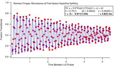
\end{figure} The signal is the Failed to parse (MathML with SVG or PNG fallback (recommended for modern browsers and accessibility tools): Invalid response ("Math extension cannot connect to Restbase.") from server "https://wikimedia.org/api/rest_v1/":): {\displaystyle {\bf{\hat e}} _z} component of the spin after the second interaction. The signal after the second Failed to parse (MathML with SVG or PNG fallback (recommended for modern browsers and accessibility tools): Invalid response ("Math extension cannot connect to Restbase.") from server "https://wikimedia.org/api/rest_v1/":): {\displaystyle \pi/2} pulse is an oscillating signal in Failed to parse (MathML with SVG or PNG fallback (recommended for modern browsers and accessibility tools): Invalid response ("Math extension cannot connect to Restbase.") from server "https://wikimedia.org/api/rest_v1/":): {\displaystyle T\delta} , depending on how much phase the spin has acquired relative to the local oscillator (the microwave signal generator at frequency Failed to parse (MathML with SVG or PNG fallback (recommended for modern browsers and accessibility tools): Invalid response ("Math extension cannot connect to Restbase.") from server "https://wikimedia.org/api/rest_v1/":): {\displaystyle \omega} ). Examples of such curves are shown in Figures \ref{fig:ramsey_signal} and \ref{fig:ramsey_vs_freq}. \begin{figure}
\caption{Ramsey oscillation signal as a function of time taken in the Vuleti\'{c} lab in 2007. The drive field was deliberately detuned from resonance so that the oscillation at the detuning frequency would be visible.}
\end{figure} \begin{figure}
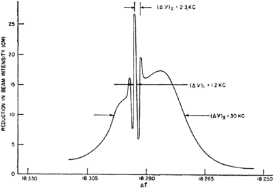
\caption{Experimental data from Ramsey's original paper \cite{Ramsey1950}, showing the signal as a function of frequency. Note the narrow oscillation, whose width is set by the measurement time Failed to parse (MathML with SVG or PNG fallback (recommended for modern browsers and accessibility tools): Invalid response ("Math extension cannot connect to Restbase.") from server "https://wikimedia.org/api/rest_v1/":): {\displaystyle T} , superimposed on the much broader background set up by the inhomogeneously broadened Failed to parse (MathML with SVG or PNG fallback (recommended for modern browsers and accessibility tools): Invalid response ("Math extension cannot connect to Restbase.") from server "https://wikimedia.org/api/rest_v1/":): {\displaystyle \pi/2} pulses.}
\end{figure} At the zero crossings we have maximum sensitivity of the signal with respect to frequency changes. Note that the signal as a function of Failed to parse (MathML with SVG or PNG fallback (recommended for modern browsers and accessibility tools): Invalid response ("Math extension cannot connect to Restbase.") from server "https://wikimedia.org/api/rest_v1/":): {\displaystyle T} looks similar to Rabi flopping. However, there the zero crossing measure the Rabi frequency, not Failed to parse (MathML with SVG or PNG fallback (recommended for modern browsers and accessibility tools): Invalid response ("Math extension cannot connect to Restbase.") from server "https://wikimedia.org/api/rest_v1/":): {\displaystyle \delta=\omega-\omega_0} .
Decoherence Processes, Mixed States, Density Matrix
The purely Hamiltonian evolution described by the Schrodinger Equation leaves the system in a pure state. However, often we have to deal with incoherent processes such as the uncontrolled loss or addition of atoms, or other perturbations that change the system evolution in an uncontrollable way. If the incoherent process is merely a (state-dependent) loss of atoms to a third state then we can describe the system by a Hamiltonian with complex eigenstates
- Failed to parse (MathML with SVG or PNG fallback (recommended for modern browsers and accessibility tools): Invalid response ("Math extension cannot connect to Restbase.") from server "https://wikimedia.org/api/rest_v1/":): {\displaystyle E_{g,e}\rightarrow E_{g,e}+i\frac{\Gamma_{g,e}t}{2} }
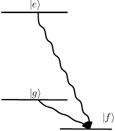
The decay of the norm Failed to parse (MathML with SVG or PNG fallback (recommended for modern browsers and accessibility tools): Invalid response ("Math extension cannot connect to Restbase.") from server "https://wikimedia.org/api/rest_v1/":): {\displaystyle \left\langle \psi\vert\psi\right\rangle } corresponds to decay out of the Failed to parse (MathML with SVG or PNG fallback (recommended for modern browsers and accessibility tools): Invalid response ("Math extension cannot connect to Restbase.") from server "https://wikimedia.org/api/rest_v1/":): {\displaystyle \left|g\right\rangle } , Failed to parse (MathML with SVG or PNG fallback (recommended for modern browsers and accessibility tools): Invalid response ("Math extension cannot connect to Restbase.") from server "https://wikimedia.org/api/rest_v1/":): {\displaystyle \left|e\right\rangle } system, as in figure \ref{fig:decay_out}. \begin{figure}
\caption{Decay out of the Failed to parse (MathML with SVG or PNG fallback (recommended for modern browsers and accessibility tools): Invalid response ("Math extension cannot connect to Restbase.") from server "https://wikimedia.org/api/rest_v1/":): {\displaystyle \left|e\right\rangle} Failed to parse (MathML with SVG or PNG fallback (recommended for modern browsers and accessibility tools): Invalid response ("Math extension cannot connect to Restbase.") from server "https://wikimedia.org/api/rest_v1/":): {\displaystyle \left|g\right\rangle} system, which can be modelled by a non-Hermitian Hamiltonian, the imaginary part of the eigenvalue corresponding to a decay rate.}
\end{figure} However, other processes, such as spontaneous decay from Failed to parse (MathML with SVG or PNG fallback (recommended for modern browsers and accessibility tools): Invalid response ("Math extension cannot connect to Restbase.") from server "https://wikimedia.org/api/rest_v1/":): {\displaystyle \left|e\right\rangle } to Failed to parse (MathML with SVG or PNG fallback (recommended for modern browsers and accessibility tools): Invalid response ("Math extension cannot connect to Restbase.") from server "https://wikimedia.org/api/rest_v1/":): {\displaystyle \left|g\right\rangle } or loss of coherence (well-defined phase relationship) between Failed to parse (MathML with SVG or PNG fallback (recommended for modern browsers and accessibility tools): Invalid response ("Math extension cannot connect to Restbase.") from server "https://wikimedia.org/api/rest_v1/":): {\displaystyle \left|e\right\rangle } and Failed to parse (MathML with SVG or PNG fallback (recommended for modern browsers and accessibility tools): Invalid response ("Math extension cannot connect to Restbase.") from server "https://wikimedia.org/api/rest_v1/":): {\displaystyle \left|g\right\rangle } due to uncontrolled level shifts (e.g. collisions, uncontrolled B-field fluctuations) cannot be dealt with within the Hamiltonian approach and require the density matrix formalism.
Density Operator
The density operator formalism is necessary when the preparation process does not prepare a single quantum state Failed to parse (MathML with SVG or PNG fallback (recommended for modern browsers and accessibility tools): Invalid response ("Math extension cannot connect to Restbase.") from server "https://wikimedia.org/api/rest_v1/":): {\displaystyle \left|\psi\right\rangle } , but a statistical mixture of quantum states Failed to parse (MathML with SVG or PNG fallback (recommended for modern browsers and accessibility tools): Invalid response ("Math extension cannot connect to Restbase.") from server "https://wikimedia.org/api/rest_v1/":): {\displaystyle \left|\psi_i\right\rangle } with probabilities Failed to parse (MathML with SVG or PNG fallback (recommended for modern browsers and accessibility tools): Invalid response ("Math extension cannot connect to Restbase.") from server "https://wikimedia.org/api/rest_v1/":): {\displaystyle P_i} . The density operator is the projection operator for that statistical mixture, or ensemble average.
- Failed to parse (MathML with SVG or PNG fallback (recommended for modern browsers and accessibility tools): Invalid response ("Math extension cannot connect to Restbase.") from server "https://wikimedia.org/api/rest_v1/":): {\displaystyle \hat{\rho}=\Sigma P_i \left|\psi_i\right\rangle \left\langle \psi_i\right| =\overline{ \left|\psi\right\rangle \left\langle \psi\right| } }
From the Schrodinger equation it follows that the Hamiltonian evolution of the density operator is governed by
- Failed to parse (MathML with SVG or PNG fallback (recommended for modern browsers and accessibility tools): Invalid response ("Math extension cannot connect to Restbase.") from server "https://wikimedia.org/api/rest_v1/":): {\displaystyle i\hbar\dot{\hat{\rho}}=\left[\hat H,\hat\rho\right] }
In the presence of damping and decay processes there are additional terms, and the time evolution is governed by a so-called Master equation. The expectation value of any operator is given by
- Failed to parse (MathML with SVG or PNG fallback (recommended for modern browsers and accessibility tools): Invalid response ("Math extension cannot connect to Restbase.") from server "https://wikimedia.org/api/rest_v1/":): {\displaystyle \left\langle \hat O\right\rangle = Tr \left(\hat O\hat \rho\right)= Tr \left(\hat \rho\hat O\right) }
The expectation value of the unity operator must be 1, so Failed to parse (MathML with SVG or PNG fallback (recommended for modern browsers and accessibility tools): Invalid response ("Math extension cannot connect to Restbase.") from server "https://wikimedia.org/api/rest_v1/":): {\displaystyle Tr \left(\hat\rho\right)=1} The expectation value of Failed to parse (MathML with SVG or PNG fallback (recommended for modern browsers and accessibility tools): Invalid response ("Math extension cannot connect to Restbase.") from server "https://wikimedia.org/api/rest_v1/":): {\displaystyle \hat\rho} , Failed to parse (MathML with SVG or PNG fallback (recommended for modern browsers and accessibility tools): Invalid response ("Math extension cannot connect to Restbase.") from server "https://wikimedia.org/api/rest_v1/":): {\displaystyle Tr \left(\hat \rho^2\right)} , is unity for a pure state , and Failed to parse (MathML with SVG or PNG fallback (recommended for modern browsers and accessibility tools): Invalid response ("Math extension cannot connect to Restbase.") from server "https://wikimedia.org/api/rest_v1/":): {\displaystyle <1} for a mixed state. In any basis , is specified in terms of its matrix elements
and the expectation value of any operator can be written as
- Failed to parse (MathML with SVG or PNG fallback (recommended for modern browsers and accessibility tools): Invalid response ("Math extension cannot connect to Restbase.") from server "https://wikimedia.org/api/rest_v1/":): {\displaystyle \begin{align} \left\langle \hat O\right\rangle &= Tr \left(\hat O\hat\rho\right) =\Sigma_n \left\langle n\right| \hat O\hat \rho \left|n\right\rangle =\Sigma_{n^\prime n} \left\langle n\right| \hat O \left|n^\prime\right\rangle \left\langle n^\prime\right| \hat \rho \left|n\right\rangle \\ \left\langle \hat O\right\rangle &= \Sigma_{nn^\prime}O_{nn^\prime}\rho_{n^\prime n} \text{ with } O_{nn^\prime}= \left\langle n\right| \hat O \left|n^\prime\right\rangle \end{align}}
The diagonal elements of the density matrix (Failed to parse (MathML with SVG or PNG fallback (recommended for modern browsers and accessibility tools): Invalid response ("Math extension cannot connect to Restbase.") from server "https://wikimedia.org/api/rest_v1/":): {\displaystyle \rho_{n^\prime n}} ) are called the probabilities since Failed to parse (MathML with SVG or PNG fallback (recommended for modern browsers and accessibility tools): Invalid response ("Math extension cannot connect to Restbase.") from server "https://wikimedia.org/api/rest_v1/":): {\displaystyle \rho_{nn}} is the probability to find the system in state Failed to parse (MathML with SVG or PNG fallback (recommended for modern browsers and accessibility tools): Invalid response ("Math extension cannot connect to Restbase.") from server "https://wikimedia.org/api/rest_v1/":): {\displaystyle n} , while the off-diagonal elements are called coherences ( is the coherence between states Failed to parse (MathML with SVG or PNG fallback (recommended for modern browsers and accessibility tools): Invalid response ("Math extension cannot connect to Restbase.") from server "https://wikimedia.org/api/rest_v1/":): {\displaystyle n^\prime} and Failed to parse (MathML with SVG or PNG fallback (recommended for modern browsers and accessibility tools): Invalid response ("Math extension cannot connect to Restbase.") from server "https://wikimedia.org/api/rest_v1/":): {\displaystyle n} ). If we write Failed to parse (MathML with SVG or PNG fallback (recommended for modern browsers and accessibility tools): Invalid response ("Math extension cannot connect to Restbase.") from server "https://wikimedia.org/api/rest_v1/":): {\displaystyle \rho_{n^\prime n}=Ae^{i\phi}} with Failed to parse (MathML with SVG or PNG fallback (recommended for modern browsers and accessibility tools): Invalid response ("Math extension cannot connect to Restbase.") from server "https://wikimedia.org/api/rest_v1/":): {\displaystyle A} , real then Failed to parse (MathML with SVG or PNG fallback (recommended for modern browsers and accessibility tools): Invalid response ("Math extension cannot connect to Restbase.") from server "https://wikimedia.org/api/rest_v1/":): {\displaystyle \phi_{n^\prime n}} is the phase between states Failed to parse (MathML with SVG or PNG fallback (recommended for modern browsers and accessibility tools): Invalid response ("Math extension cannot connect to Restbase.") from server "https://wikimedia.org/api/rest_v1/":): {\displaystyle n^\prime} and Failed to parse (MathML with SVG or PNG fallback (recommended for modern browsers and accessibility tools): Invalid response ("Math extension cannot connect to Restbase.") from server "https://wikimedia.org/api/rest_v1/":): {\displaystyle n} , while Failed to parse (MathML with SVG or PNG fallback (recommended for modern browsers and accessibility tools): Invalid response ("Math extension cannot connect to Restbase.") from server "https://wikimedia.org/api/rest_v1/":): {\displaystyle A\leq\sqrt{\rho_{nn}\rho_{n^\prime n^\prime}}} . The coherence is maximum when . Finally note that the density operator is hermitian, so that Failed to parse (MathML with SVG or PNG fallback (recommended for modern browsers and accessibility tools): Invalid response ("Math extension cannot connect to Restbase.") from server "https://wikimedia.org/api/rest_v1/":): {\displaystyle \rho_{n^\prime n} = {\rho_nn^\prime}^\star} , as we would expect for a meaningfully-defined coherence between two states.
Density Matrix for a Two-Level System and Bloch Vector
We now introduce a slightly different parametrization of the two-level Hamiltonian \ref{eq:dressed_atom_hamiltonian} and of the corresponding density matrix:
- Failed to parse (MathML with SVG or PNG fallback (recommended for modern browsers and accessibility tools): Invalid response ("Math extension cannot connect to Restbase.") from server "https://wikimedia.org/api/rest_v1/":): {\displaystyle \begin{align} H&= \frac{\hbar}{2} \begin{pmatrix} \omega_0 & \omega_R e^{-i\omega t} \\ \omega_R e^{i \omega t} & -\omega_0 \end{pmatrix} =\frac{\hbar}{2} \begin{pmatrix} \omega_0 & V_1-iV_2 \\ V_1+iV_2 & -\omega_0 \end{pmatrix} \\ &= \frac{\hbar}{2} \left(V_1\hat\sigma_x+V_2\hat\sigma_y+\omega_0\hat\sigma_z\right) \\ \rho&= \begin{pmatrix} \rho_{11} & \rho_{12} \\ \rho_{21} & \rho_{22} \end{pmatrix} =\frac{1}{2} \begin{pmatrix} r_0+r_3 & r_1-ir_2 \\ r_1+ir_2 & r_0-r_3 \end{pmatrix} \\ &= \frac{1}{2} \left(r_0\hat 1 + r_1\hat\sigma_x + r_2\hat\sigma_y + r_3 \hat\sigma_z\right) \end{align}}
In the problem set you will show (or have shown) that the Hamiltonian evolution of the density matrix
- Failed to parse (MathML with SVG or PNG fallback (recommended for modern browsers and accessibility tools): Invalid response ("Math extension cannot connect to Restbase.") from server "https://wikimedia.org/api/rest_v1/":): {\displaystyle i\hbar\dot \rho=\left[H_1,\rho\right] }
implies the equation of motion
- Failed to parse (MathML with SVG or PNG fallback (recommended for modern browsers and accessibility tools): Invalid response ("Math extension cannot connect to Restbase.") from server "https://wikimedia.org/api/rest_v1/":): {\displaystyle \frac{d {\bf{r}} }{dt} = {\bf{\omega}} \times {\bf{r}} }
for the vectors and Failed to parse (MathML with SVG or PNG fallback (recommended for modern browsers and accessibility tools): Invalid response ("Math extension cannot connect to Restbase.") from server "https://wikimedia.org/api/rest_v1/":): {\displaystyle {\bf{\omega}} =\left(V_1,V_2,\omega_0\right)} This slightly generalizes our previous result: for a pure state using the Heisenberg equations of motion we had shown that the spin-Failed to parse (MathML with SVG or PNG fallback (recommended for modern browsers and accessibility tools): Invalid response ("Math extension cannot connect to Restbase.") from server "https://wikimedia.org/api/rest_v1/":): {\displaystyle 1/2} and the corresponding magnetic moment obey
- Failed to parse (MathML with SVG or PNG fallback (recommended for modern browsers and accessibility tools): Invalid response ("Math extension cannot connect to Restbase.") from server "https://wikimedia.org/api/rest_v1/":): {\displaystyle \frac{d {\bf{S}} }{dt}= {\bf{\omega}} \times {\bf{S}} }
but we have now generalized this result to mixed states, i.e. to ensemble averages that have less than the maximum possible magnetic moment. Note that Hamiltonian evolution does not change the purity of a state: a pure state always remains pure, no matter how violently it is rotated, and a mixed state retains its degree of mixedness (Failed to parse (MathML with SVG or PNG fallback (recommended for modern browsers and accessibility tools): Invalid response ("Math extension cannot connect to Restbase.") from server "https://wikimedia.org/api/rest_v1/":): {\displaystyle Tr \rho^2(t)=\text{const.}} ) Here we can check this explicitly by noting that
Since Failed to parse (MathML with SVG or PNG fallback (recommended for modern browsers and accessibility tools): Invalid response ("Math extension cannot connect to Restbase.") from server "https://wikimedia.org/api/rest_v1/":): {\displaystyle \dot{ {\bf{r}} }\perp {\bf{r}} } , the length of Failed to parse (MathML with SVG or PNG fallback (recommended for modern browsers and accessibility tools): Invalid response ("Math extension cannot connect to Restbase.") from server "https://wikimedia.org/api/rest_v1/":): {\displaystyle {\bf{r}} } does not change, and hence Failed to parse (MathML with SVG or PNG fallback (recommended for modern browsers and accessibility tools): Invalid response ("Math extension cannot connect to Restbase.") from server "https://wikimedia.org/api/rest_v1/":): {\displaystyle Tr \rho^2} is constant in time.









![{\displaystyle {\frac {d}{dt}}{\hat {O}}={\frac {i}{\hbar }}\left[{\hat {H}},{\hat {O}}\right]+{\frac {\partial {\hat {O}}}{\partial t}}}](https://wikimedia.org/api/rest_v1/media/math/render/svg/ae5069cad777556e25ef2674f2ed7f1fbdc641a0)
![{\displaystyle {\frac {d}{dt}}{\hat {\mu }}_{k}=\gamma {\frac {d}{dt}}{\hat {L}}_{k}={\frac {i\gamma }{\hbar }}\left[{\hat {H}},{\hat {L}}_{k}\right]=-{\frac {i\gamma ^{2}}{\hbar }}B_{0}\left[{\hat {L}}_{z},{\hat {L}}_{k}\right]}](https://wikimedia.org/api/rest_v1/media/math/render/svg/31c5220d2321caf92920986550a99c6ba69fb523)
![{\displaystyle \left[{\hat {L}}_{k},{\hat {L}}_{l}\right]=i\hbar \epsilon _{klm}{\hat {L}}_{m}}](https://wikimedia.org/api/rest_v1/media/math/render/svg/5b0dce00bc29fe901e80ab62151d3d46ed0adb58)


