Difference between revisions of "Quantized spin in a magnetic field"
imported>Ketterle |
imported>Ketterle |
||
| Line 252: | Line 252: | ||
as already derived from the fact that the expectation value for | as already derived from the fact that the expectation value for | ||
the magnetic moment obeys the classical equation. | the magnetic moment obeys the classical equation. | ||
| + | |||
| + | |||
| + | |||
| + | |||
| + | The quantum mechanical treatment yields a probability for non-adiabatic transition (probability for the | ||
| + | magnetic moment not following the magnetic field) given by | ||
| + | :<math> | ||
| + | P_\text{na}=exp\left(-\frac{\pi}{2}\frac{\omega^2_R}{ \left| \dot\omega\right| }\right) | ||
| + | </math> | ||
| + | in agreement with the qualitative classical criterion derived above. | ||
=== Atomic Clocks and the Ramsey Method === | === Atomic Clocks and the Ramsey Method === | ||
Revision as of 14:47, 17 February 2010
Contents
Equation of Motion for the Expectation Value
For the system we have been considering, the Hamiltonian is
Recalling the Heisenberg equation of motion for any operator is
where the last term refers to operators with an explicit time dependence, we have in this instance
Using with the Levi-Civita symbol , we have
or in short
These are just like the classical equations of motion \ref{eq:classical_precession_in_static_field}, but here they describe the precession of the operator for the magnetic moment or for the angular momentum about the magnetic field at the (Larmor) angular frequency .
Note that:
- Just as in the classical model, these operator equations are exact; we have not neglected any higher order terms.
- Since the equations of motion hold for the operator, they must hold for the expectation value
- We have not made use of any special relations for a spin- system, but just the general commutation relation for angular momentum. Therefore the result, precession about the magnetic field at the Larmor frequency, remains true for any value of angular momentum .
- A spin- system has two energy levels, and the two-level problem with coupling between two levels can be mapped onto the problem for a spin in a magnetic field, for which we have developed a good classical intuition.
- If coupling between two or more angular momenta or spins within an atom results in an angular momentum , the time evolution of this angular momentum in an external field is governed by the same physics as for the two-level system. This is true as long as the applied magnetic field is not large enough to break the coupling between the angular momenta; a situation known as the Zeeman regime. Note that if the coupled angular momenta have different gyromagnetic ratios, the gyromagnetic ratio for the composite angular momentum is different from those of the constituents.
- For large magnetic field the interaction of the individual constituents with the magnetic field dominates, and they precess separately about the magnetic field. This is the Paschen-Back regime.
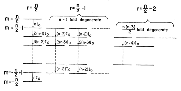
- An even more interesting composite angular momentum arises when two-level atoms are coupled symmetrically to an external field. In this case we have an effective angular momentum for the symmetric coupling:
Level structure diagram for two-level atoms in a basis of symmetric states \cite{Dicke1954}. The leftmost column corresponds to an effective spin- object. Other columns correspond to manifolds of symmetric states of the atoms with lower total effective angular momentum.
- Again the equation of motion for the composite angular momentum is a precession. This is the problem considered in Dicke's famous paper \cite{Dicke1954}, in which he shows that this collective precession can give rise to massively enhanced couplings to external fields ("superradiance") due to constructive interference between the individual atoms.
The Two-Level System: Spin-1/2
Let us now specialize to the two-level system and calculate the time evolution of the occupation probabilities for the two levels.
Equivalence of two-level system with spin-. Note that for the spin-up state (spin aligned with field) is the ground state. For an electron, with , spin-up is the excited state. Be careful, as both conventions are used in the literature.
We have that
where in the last equation we have used the fact that . The signs are chosen for a spin with , such as a proton (Figure \ref{fig:two_level_spin_half}). For an electron, or any other spin with , the analysis would be the same but for the opposite sign of and the corresponding exchange of and . If the system is initially in the ground state, (or the spin along , ), the expectation value obeys the classical equation of motion \ref{eq:classical_rabi_flopping}:
- {eqn:rabi_transition_probability}
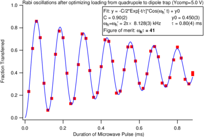
Equation \ref{eqn:rabi_transition_probability} is the probability to find system in the excited state at time if it was in ground state at time . Figure \ref{fig:rabi_signal} shows a real-world example of such an oscillation.
{fig:rabi_signal} Rabi oscillation signal taken in the Vuleti\'{c} lab shortly after this topic was covered in lecture in 2008. The amplitude of the oscillations decays with time due to spatial variations in the strength of the drive field (and hence of the Rabi frequency), so that the different atoms drift out of phase with each other.
Matrix form of Hamiltonian
With the matrix representation
we can write the Hamiltonian associated with the static field as
where is the Larmor frequency, and
is a Pauli spin matrix. The eigenstates are , with eigenenergies . A spin initially along , corresponding to
evolves in time as
which describes a precession with angluar frequency . The field , rotating at in the plane corresponds to
where have used the Pauli spin matrices , . The full Hamiltonian is thus given by
This is the famous "dressed atom" Hamiltonian in the so-called "rotating wave approximation". Its eigenstates and eigenvalues provide a very elegant, very intuitive solution to the two-state problem.
Solution of the Schrodinger Equation for Spin-1/2 in the Interaction Representation
The interaction representation consists of expanding the state in terms of the eigenstates , of the Hamiltonian , including their known time dependence due to . That means we write here
Substituting this into the Schrodinger equation
then results in the equations of motion for the coefficients
Where we have used the matrix form of the Hamiltonian, \ref{eq:dressed_atom_hamiltonian}. Introducing the detuning , we have
The explicit time dependence can be eliminated by the sustitution
As you will show (or have shown) in the problem set, this leads to solutions for given by
with two constants that are determined by the initial conditions. For we find
as already derived from the fact that the expectation value for the magnetic moment obeys the classical equation.
The quantum mechanical treatment yields a probability for non-adiabatic transition (probability for the
magnetic moment not following the magnetic field) given by
in agreement with the qualitative classical criterion derived above.
Atomic Clocks and the Ramsey Method
When comparing the Hamiltonian for a spin- in a magnetic field to that of a two-level system with a coupling between the two levels characterized by the strength and frequency , we see that the energy spacing between and corresponds to the Larmor frequency in the static field. This spacing can provide a frequency or time reference if perturbations affecting are sufficiently well controlled. For instance, the time unit "second" is defined via the transition frequency between two hyperfine states in the electronic ground state of the caesium atom, which is near Failed to parse (unknown function "\unit"): {\displaystyle \unit{9.2}{\giga\hertz}} in the microwave domain. The task of an atomic clock is then to measure this frequency accurately by trying to tune a frequency source (the frequency of the rotating field in the spin picture) to the atomic frequency . Equivalently, we want to find the frequency such that the detuning is equal to zero. Starting with an atom in (spin along for ), we could try to find the resonance frequency by noting that according to
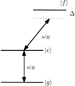
the population of the upper state is maximized for (i.e. the precession of the spin to the direction is only complete on resonance). This is the so-called Rabi method. It suffers from a number of drawbacks. For one, the signal is only quadratic in the detuning , i.e. the method is relatively insensitive near . Furthermore, the optimum time depends on the strength of the coupling (i.e. the strength of the rotating field), so fluctuations in can be mistaken for changes in . Finally the coupling by to other levels can lead to level shifts that are not intrinsic to the atom, but depend on the applied drive (Figure \ref{fig:rabi_third_level}).
{fig:rabi_third_level} The drive used for Rabi flopping within the , system can also off-resonantly couple one or both levels to other states, perturbing the transition frequency .
Norman Ramsey invented an alternative method (the so-called "separated oscillatory fields method", known for short as the "Ramsey method" \cite{Ramsey1949,Ramsey1950}, for which he received the Nobel prize), that fixes all of these problems. It leads to a signal that is linear rather than quadratic in the detuning , does not require tuning the measurement time to match the applied field strength , and, most importantly, eliminates level shifts due to altogether. The method is as follows. Instead of applying a pulse for a time t that corresponds to Rabi rotation of the spin by (called a pulse), the pulse is applied for half that time, corresponding to the Rabi rotation of the spin by into the plane ( pulse). Then the applied field is turned off and the system is left to precess in the static field (or at its natural frequency ) for a measurement time . Finally, a second pulse, identical to the original one, is applied (see Figure \ref{fig:ramsey_sequence}).
{fig:ramsey_sequence} Ramsey sequence
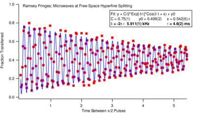
The signal is the component of the spin after the second interaction. The signal after the second pulse is an oscillating signal in , depending on how much phase the spin has acquired relative to the local oscillator (the microwave signal generator at frequency ). Examples of such curves are shown in Figures \ref{fig:ramsey_signal} and \ref{fig:ramsey_vs_freq}.
{fig:ramsey_signal} Ramsey oscillation signal as a function of time taken in the Vuleti\'{c} lab in 2007. The drive field was deliberately detuned from resonance so that the oscillation at the detuning frequency would be visible.
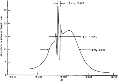
{fig:ramsey_vs_freq} Experimental data from Ramsey's original paper \cite{Ramsey1950}, showing the signal as a function of frequency. Note the narrow oscillation, whose width is set by the measurement time , superimposed on the much broader background set up by the inhomogeneously broadened pulses.
At the zero crossings we have maximum sensitivity of the signal with respect to frequency changes. Note that the signal as a function of looks similar to Rabi flopping. However, there the zero crossing measure the Rabi frequency, not .


![{\displaystyle {\frac {d}{dt}}{\hat {O}}={\frac {i}{\hbar }}\left[{\hat {H}},{\hat {O}}\right]+{\frac {\partial {\hat {O}}}{\partial t}}}](https://wikimedia.org/api/rest_v1/media/math/render/svg/ae5069cad777556e25ef2674f2ed7f1fbdc641a0)
![{\displaystyle {\frac {d}{dt}}{\hat {\mu }}_{k}=\gamma {\frac {d}{dt}}{\hat {L}}_{k}={\frac {i\gamma }{\hbar }}\left[{\hat {H}},{\hat {L}}_{k}\right]=-{\frac {i\gamma ^{2}}{\hbar }}B_{0}\left[{\hat {L}}_{z},{\hat {L}}_{k}\right]}](https://wikimedia.org/api/rest_v1/media/math/render/svg/31c5220d2321caf92920986550a99c6ba69fb523)
![{\displaystyle \left[{\hat {L}}_{k},{\hat {L}}_{l}\right]=i\hbar \epsilon _{klm}{\hat {L}}_{m}}](https://wikimedia.org/api/rest_v1/media/math/render/svg/5b0dce00bc29fe901e80ab62151d3d46ed0adb58)


