Derivation of the optical Bloch equations

The master equation is an equation of motion for a density matrix describing an open quantum system, much like the Schrodinger equation describes the evolution of a closed quantum system. This section provides a derivation of the master equation for a spontaneously emitting atom, driven by a classical field, which is known as the Optical Bloch Equation.

▼ Category:8.422

► Category:Quantum Light

► Category:Optical Bloch Equations

► Category:Bose-Einstein condensates

► Category:Ion traps and quantum information

► Category:Light forces

► Category:Photon-atom interactions

  Introduction to Atomic Physics

  Quantum light: states and dynamics

  Optical Bloch equations

  Photon-atom interactions

  Frontiers in Atomic Physics

  Ion traps and quantum information

  Quantum gases

Classical model of atom and field

A good starting point, to appreciate the problem of open quantum systems, is the classical model for a two-level atom coupled to a black-body electromagnetic field, the Einstein rate equations

${\begin{array}{rcl}{\frac {dN_{g}}{dt}}&=&A_{eg}N_{e}+u(\omega _{eg})\left[{B_{eg}N_{e}-B_{ge}N_{g}}\right]\\{\frac {dN_{e}}{dt}}&=&-A_{eg}N_{e}+u(\omega _{eg})\left[{B_{ge}N_{g}-B_{eg}N_{e}}\right]\,,\end{array}}$

where $A_{eg}$ is the spontaneous emission rate, $B_{ge}$ and $B_{eg}$ are stimulated emission rates, and $u(\omega _{eg})$ is the field energy density at atomic frequency $\omega _{eg}$, for levels denoted by $|e{\rangle }$ and $|g{\rangle }$.

Is there a straightforward quantum analogue of this? We might be tempted to simply add a damping term to the Schrödinger equation, like

$i\hbar \partial _{t}|\psi \rangle =H|\psi \rangle -i\Gamma |\psi {\rangle }\,,$

but this is not physically allowed by quantum mechanics! How, then, can we construct a fully quantum-mechanical description of open system dynamics? The key concept is that we must properly account for noise:

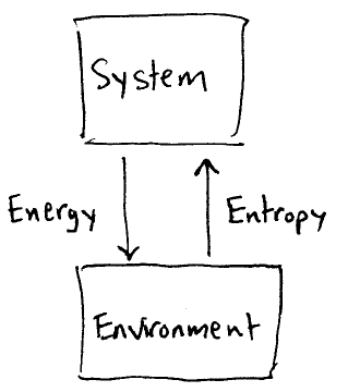
From classical thermodynamics, we know that any time there is energy transfer from a system to the environment, there is entropy exchanged back from the environment to the system. This is a simple illustration of the very basic fluctuation--dissipation principle: there can be no relaxation without con-commitment noise! To study quantum open system, we must model the appropriate quantum noise contribution which goes along with relaxation.

Density matrices and closed system dynamics

The main tool we shall use to model open quantum systems is the density matrix representation for quantum states, so it is helpful to begin with a review of density matrices and how they evolve under Hamiltonian dynamics.

Review of density matrices: definition, properties, and unravlings

Recall that a density matrix $\rho$ for a pure state $|\psi {\rangle }$ is the matrix $|\psi {\rangle }{\langle }\psi |$. Thus, for example

${\begin{array}{rcl}|0\rangle &\rightarrow &\left[{\begin{array}{cc}{1}&{0}\\{0}&{0}\end{array}}\right]\\&&~\\|1\rangle &\rightarrow &\left[{\begin{array}{cc}{0}&{0}\\{0}&{1}\end{array}}\right]\\&&~\\{\frac {|0{\rangle }+|1{\rangle }}{\sqrt {2}}}&\rightarrow &{\frac {1}{2}}\left[{\begin{array}{cc}{1}&{1}\\{1}&{1}\end{array}}\right]\,.\end{array}}$

Density matrices may also represent statistical mixtures of pure states; this state

${\frac {1}{2}}\left[{\begin{array}{cc}{1}&{0}\\{0}&{1}\end{array}}\right]$

can be interpreted as a 50/50 mixture of $|0{\rangle }$ and $|1{\rangle }$. However, one must be careful, because there are infinitely many ways to unravel a density matrix into statistical mixtures of pure states.

For example,

$\rho ={\frac {1}{4}}\left[{\begin{array}{cc}{3}&{0}\\{0}&{1}\end{array}}\right]$

is

$\rho ={\frac {3}{4}}|0\rangle \langle 0|+{\frac {1}{4}}|1\rangle \langle 1|\,,$

but it is also

$\rho ={\frac {1}{2}}|a\rangle \langle a|+{\frac {1}{2}}|b\rangle \langle b|\,,$

where

${\begin{array}{rcl}|a\rangle &=&{\frac {{\sqrt {3}}|0{\rangle }+|1{\rangle }}{2}}\\|b\rangle &=&{\frac {{\sqrt {3}}|0{\rangle }-|1{\rangle }}{2}}\,.\end{array}}$

In general, a density matrix $\rho$ may always be written as a statistical mixture of pure states,

$\rho =\sum _{k}p_{k}|\psi _{k}{\rangle }\,,$

where $p_{k}$ are probabilities, such that $\sum _{k}p_{k}=1$.

A matrix $\rho$ is a valid density matrix if and only if the eigenvalues of $\rho$ are non-negative, and sum to one, such that ${\rm {Tr}}(\rho )=1$. $\rho$ represents a pure state if and only if ${\rm {Tr}}(\rho ^{2})=1$.

Density matrices: closed system evolution

How does a density matrix evolve in a closed system? From the Schrodinger equation

$i\hbar \partial _{t}|\psi \rangle =H|\psi {\rangle }\,,$

it follows that a pure state density matrix $\rho =|\psi {\rangle }{\langle }\psi |$ evolves as

${\begin{array}{rcl}{\dot {\rho }}&=&|{\dot {\psi }}{\rangle }{\langle }\psi |+|\psi {\rangle }{\langle }{\dot {\psi }}|\\&=&-{\frac {i}{\hbar }}[H,\rho ]\,.\end{array}}$

For example, if $\rho$ is a two-level atom evolving under the classical field Jaynes-Cummings Hamiltonian

$H={\frac {\hbar \omega _{0}}{2}}(|e\rangle \langle e|-|g\rangle \langle g|)+\Omega (|g\rangle \langle e|+|e\rangle \langle g|)\,,$

which we may express using Pauli matrices as

$H={\frac {\hbar \omega _{0}}{2}}Z+\Omega X\,,$

then for

$\rho =\left[{\begin{array}{cc}{\rho _{ee}}&{\rho _{eg}}\\{\rho _{ge}}&{\rho _{gg}}\end{array}}\right]\,,$

the equation of motion for $\rho$ is

${\dot {\rho }}=\left[{\begin{array}{cc}{i\Omega (\rho _{eg}-\rho _{ge})}&{i\omega _{0}\rho _{ge}-i\Omega (\rho _{ee}-\rho _{gg})}\\{-i\omega _{0}\rho _{eg}+i\Omega (\rho _{ee}-\rho _{gg})}&{i\Omega (\rho _{eg}-\rho _{ge})}\end{array}}\right]\,.$

We can recognize this as a rotation of the Bloch sphere about the axis defined by

${\vec {n}}={\frac {\hbar \omega _{0}}{2}}{\hat {z}}+\Omega {\hat {x}}\,,$

by using the Bloch sphere representation for a density matrix,

$\rho ={\frac {I+{\vec {r}}\cdot {\sigma }}{2}}\,.$

Density matrices and open system dynamics: approach

We can build a mathematical model for quantum open system dynamics, based on four basic ideas:

Density matrix evolution	Instead of pure states (eg $|\psi {\rangle }$), we describe the system state using a density matrix $\rho$. The equation of motion for $\rho$ is ${\dot {\rho }}={\mathcal {L}}[\rho ]\,,$ where ${\mathcal {L}}$ is known as the Liouvillian operator (or a "superoperator"). For example, for Hamiltonian evolution, we have: $i\hbar \partial _{t}|\psi \rangle =H|\psi {\rangle }$ which, for $\rho =|\psi {\rangle }{\langle }\psi |$ gives ${\begin{array}{rcl}\partial _{t}\rho &=&|{\dot {\psi }}{\rangle }{\langle }\psi |+|\psi {\rangle }{\langle }{\dot {\psi }}|\\&=&-{\frac {i}{\hbar }}H|\psi {\rangle }{\langle }\psi |+|\psi {\rangle }{\langle }\psi |{\frac {i}{\hbar }}H\\&=&-{\frac {i}{\hbar }}[H,\rho ]\,.\end{array}}$ This is unitary evolution, but in general, the differential equation for $\rho$ can describe non-unitary evolution. Such differential equations are known as "master equations." They are nontrivial to construct, because they must restrict $\rho$ to be a legitimate density matrix at all times.
Partial trace	We are interested in the state of the system alone, and want to disregard the state of the environment. If $\rho _{\rm {total}}$ is the state of the whole system + environment, then the state of the system alone is ${\begin{array}{rcl}\rho _{sys}&=&{\rm {Tr}}_{env}\left[{\rho _{\rm {total}}}\right]\\&=&\sum _{\rm {env}}{\langle }{\rm {env}}|\rho _{\rm {total}}|{\rm {env}}{\rangle }\,.\end{array}}$
Assumptions about the environment	The environment is also known as a "bath" or a "reservoir" (cf API). We model it as being an ensemble of oscillators, of a variety of frequencies, which are weakly coupled to the system. It has several important properties: Large and unchanging -- Born approximation Short correlation time $\tau _{c}$ -- Markov approximation
Two (very different) timescales	There are two important timescales in this model: $T_{relax}$: A slow evolution of the system $\tau _{c}$: The fast fluctuations of the environment We will build equations of motion which have a timescale $\Delta t$, chosen such that $\tau _{c}\ll \Delta t\ll T_{relax}$.

Our goal is to construct a model dynamical equation of motion for $\rho _{sys}$ of the form

${\frac {\Delta \rho _{sys}}{\Delta t}}=M\rho _{sys}\,,$

where $M$ is time independent. This is known as a "coarse grained" evolution equation. It is desirable to obtain $M$ for a variety of scenarios, including interactions where the system + environment are atom + light, light + light, and atom + motion, for example. Below, we construct a master equation for the atom + vacuum using two different approaches.

Beamsplitter model of the master equation

The physical intuition behind the master equation we desire to construct can be captured with a simple example, which builds on the beamsplitter we studied in previous lectures.

Single photon through beamsplitter: pure state description

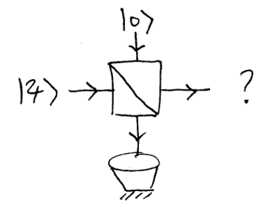
Consider a single photon state $|\psi \rangle =\alpha |0\rangle +\beta |1{\rangle }$ (for simplicity, let the coefficients be real-valued) entering a beamsplitter of angle $\theta$:

A vacuum state $|0{\rangle }$ is input to the other port, whose output we discard. Let us consider the photon as being our system, and the other (initially vacuum) mode as being our environment. What is the quantum state of the undiscarded output? Naively, we might argue that a single photon is discarded into the environment with probability $p_{1}=\beta ^{2}\sin ^{2}\theta$, so that we might expect the output to be $|0{\rangle }$ with probability $p_{1}$, and $|\psi {\rangle }$ with probability $1-p_{1}$.

However, that (semi-)classical argument is incorrect. The output state $|\phi {\rangle }$ of the system + environment is

${\begin{array}{rcl}|\phi \rangle &=&e^{i\theta (a^{\dagger }b+b^{\dagger }a)}\left[{|\psi \rangle \otimes |0\rangle }\right]\\&=&\alpha |00\rangle +\beta \left[{\cos \theta |10\rangle +\sin \theta |01\rangle }\right]\\&=&\left[{\alpha |0\rangle +\beta \cos \theta |1\rangle }\right]\otimes |0{\rangle }+\left[{\beta \sin \theta |0\rangle }\right]\otimes |1{\rangle }\,.\end{array}}$

Thus, the correct result is that the output is $|\psi _{0}\rangle =(\alpha |0\rangle +\beta \cos \theta |1\rangle )/{\sqrt {\alpha ^{2}+\beta ^{2}\cos ^{2}\theta }}$, with probability $1-p_{1}$, and $|\psi _{1}\rangle =|0{\rangle }$ with probability $p_{1}$.

Single photon through beamsplitter: density matrix description

These states can conveniently be written as density matrices. The input state is

$\rho _{in}=|\psi {\rangle }{\langle }\psi |=\left[{\begin{array}{cc}{\alpha ^{2}}&{\alpha \beta }\\{\alpha \beta }&{\beta ^{2}}\end{array}}\right]\,,$

(3.3.1)

and the output state is

${\begin{array}{rcl}\rho _{out}=p_{1}|\psi _{1}{\rangle }{\langle }\psi _{1}|+p_{0}|\psi _{0}{\rangle }{\langle }\psi _{0}|=\left[{\begin{array}{cc}{\alpha ^{2}+\beta ^{2}\sin ^{2}\theta }&{\alpha \beta \cos \theta }\\{\alpha \beta \cos \theta }&{\beta ^{2}\cos ^{2}\theta }\end{array}}\right]\,.\end{array}}$

Note that $\rho _{out}$ cannot be written as $|\chi {\rangle }{\langle }\chi |$ for any pure state $|\chi {\rangle }$, because it is not pure (it is a statistical mixture). The change in $\rho$ is

$\Delta \rho =\rho _{out}-\rho _{in}=\left[{\begin{array}{cc}{-\beta ^{2}(\cos 2\theta -1)/2}&{\alpha \beta (\cos \theta -1)}\\{\alpha \beta (\cos \theta -1)}&{\beta ^{2}(\cos 2\theta -1)/2}\end{array}}\right]\,.$

Single photon through many beamsplitters: coarse-grained evolution

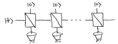
Now imagine that we send the single photon state through many beamsplitters in a sequence, each with some small tap angle $\theta ={\sqrt {\Gamma \Delta t/2}}$:

We make two assumptions: the environment modes always begin in the vacuum $|0{\rangle }$ (this is the Born approximation), and the environment is completely different and uncorrelated between scattering events (this is the Markov approximation).

This allows us to write a coarse-grained differential equation for the photon state

${\frac {\Delta \rho }{\Delta t}}\approx \left[{\begin{array}{cc}{{\dot {\rho }}_{00}}&{{\dot {\rho }}_{01}}\\{{\dot {\rho }}_{10}}&{{\dot {\rho }}_{11}}\end{array}}\right]=-\Gamma \left[{\begin{array}{cc}{-\beta ^{2}}&{\alpha \beta /2}\\{\alpha \beta /2}&{\beta ^{2}}\end{array}}\right]\,.$

Expressed as differential equations for each of the independent matrix elements, we get (using Eq.(3.3.1) for $\rho (t=0)$)

${\begin{array}{rcl}{\frac {d}{dt}}\rho _{00}&=&+\Gamma \rho _{11}\\{\frac {d}{dt}}\rho _{11}&=&-\Gamma \rho _{11}\end{array}}$

for the diagonal elements.

These describe the evolutions of the probabilities of finding the photon in the $|0{\rangle }$ and $|1{\rangle }$ states, and are analogous to the Einstein rate equations. And for the off-diagonal elements we get

${\begin{array}{rcl}{\frac {d}{dt}}\rho _{01}&=&-{\frac {\Gamma }{2}}\rho _{01}\\{\frac {d}{dt}}\rho _{10}&=&-{\frac {\Gamma }{2}}\rho _{10}\end{array}}$

which show the decay of the quantum coherence of the state.

Comparison to the general master equation

The form of these differential equations, which are master equations, is very general, and almost exactly the same result is obtained for a two-level atom interacting with the vacuum. In that situation, the solution differs essentially only in that the coherences evolve as

${\begin{array}{rcl}{\frac {d}{dt}}\rho _{01}&=&-\left({i\Delta +{\frac {\Gamma }{2}}}\right)\rho _{01}\,,\end{array}}$

where $\Delta$ is a frequency shift of the system known as the "Lamb shift," which is due to virtual excitations to higher atomic levels.

In the atomic master equation, $\Gamma$ is the spontaneous emission rate, given by Fermi's golden rule

$\Gamma ={\frac {2\pi }{\hbar }}\sum _{\kappa \epsilon }|\langle g;\kappa \epsilon |V|e;0{\rangle }|^{2}\delta (\hbar \omega -\hbar \omega _{ge})\,,$

as derived elsewhere.

Full derivation -- walk-through

We now turn to a full derivation of the general master equation.

Master equation in integral form for arbitrary interaction

Following the notation used in API, Chapter 4, let $A$ denote the system, and $R$ the environment (known as the reservoir in API). The full Hamiltonian is

$H=H_{A}+H_{R}+V\,,$

where $V$ is the system-reservoir interaction potential. In the interaction picture defined by $H_{A}$ and $H_{R}$, the equation of motion for the full system + reservoir density matrix is

$i\hbar {\dot {\rho }}=[V,\rho ]\,.$

(3.2)

Integrating this once gives

$i\hbar \rho (t)=\int _{0}^{t}[V(t'),\rho (t')]\,dt'\,.$

Substituting this back into Eq.(3.2) gives

${\dot {\rho }}=-{\frac {1}{\hbar ^{2}}}\int _{0}^{t}[V(t),[V(t'),\rho (t')]]\,dt'\,.$

If we assume that the system and reservoir are initially uncorrelated, and make the approximation that the reservoir stays unchanged (the Born approximation), then

$\rho (t)\approx \rho _{A}(t)\otimes \rho _{R}(0)=\rho _{A}(t)\otimes \rho _{R}$

This gives us our starting point for a general master equation:

${\dot {\rho }}_{A}=-{\frac {1}{\hbar ^{2}}}{\rm {Tr}}_{R}\int _{0}^{t}[V(t),[V(t'),\rho _{A}(t')\otimes \rho _{R}]]\,dt'\,.$

Master equation for a two-level atom interacting with the vacuum

An example is helpful in seeing how this equation works. Generally, we will take system + reservoir interactions of the form $V=-AR$, where $A$ acts only on the system, and $R$ acts only on the reservoir. Specifically, let the system be a two-level atom, and the environment be a single electromagnetic mode initially in the vacuum state $|0{\rangle }$. The atom interacts with the usual dipole interaction,

$V=-{\frac {\Gamma }{2}}(b^{\dagger }|g\rangle \langle e|+b|e\rangle \langle g|)\,,$

which is conveniently written using Pauli raising and lowering operators

$\sigma _{\pm }={\frac {\sigma _{x}\pm i\sigma _{y}}{2}}$

where

$\sigma _{-}=|g\rangle \langle e|~~~~~~{\rm {and}}~~~~~~\sigma _{+}=|e\rangle \langle g|\,.$

Insert this now into Eq.(\ref{eq:rhome}), but disregard the integral over time (this lets us see what the essential dynamics are, at the expense of not obtaining the correct specific rates). The relevant commutators are

$\left[{V,\rho _{A}\otimes |0\rangle \langle 0|}\right]=(\sigma _{-}\rho _{A})\otimes |1\rangle \langle 0|-(\rho _{A}\sigma _{+})\otimes |0\rangle \langle 1|$

and

$\left[{V,\left[{V,\rho _{A}\otimes |0\rangle \langle 0|}\right]}\right]=(\sigma _{+}\sigma _{-}\rho _{A})\otimes |0\rangle \langle 0|-2(\sigma _{-}\rho _{A}\sigma _{+})\otimes |1\rangle \langle 1|+(\rho _{A}\sigma _{+}\sigma _{-})|0\rangle \langle 0|+{\rm {other}}\,,$

where the "other" terms are not diagonal in the electromagnetic mode states, and thus disappear in the partial trace over the reservoir. We find, finally:

${\dot {\rho }}_{A}=-{\frac {\Gamma }{2}}\left[{\sigma _{+}\sigma _{-}\rho _{A}-2\sigma _{-}\rho _{A}\sigma _{+}+\rho _{A}\sigma _{+}\sigma _{-}}\right]\,.$

This is the master equation for a two-level atom dipole coupled to a single electromagnetic mode initially in the vacuum state. It is written in a form known as the "Lindblad" form, which is very common. In atomic physics, you will often see master equations like this.

The Lindblad form has the special property that it ensures $\rho$ is a legitimate density matrix at all times; not only does ${\rm {Tr}}(\rho )=1$ always, but also, its eigenvalues remain non-negative. And more importantly, the map from $\rho (t)$ to $\rho (t')$ is completely positive, meaning that if the map operates on just part of a larger system, the state of the larger system remains described by a valid, positive density matrix. Using the definitions for $\sigma _{\pm }$, if we express $\rho _{A}$ as

$\rho _{A}=\left[{\begin{array}{cc}{a}&{b}\\{c}&{d}\end{array}}\right]\,,$

then we find

${\dot {\rho }}_{A}=-\Gamma \left[{\begin{array}{cc}{2a}&{b}\\{c}&{-2a}\end{array}}\right]\,,$

which is identical to the master equation we constructed for the beamsplitter example, Eq.(\ref{eq:bsme}), up to a relabeling of $|g{\rangle }$ and $|e{\rangle }$.

As shown by this example, the physical picture behind the master equation is not so complicated, even though the mathematics (used in all its glory) can be overwhelming.

Putting it together: the optical Bloch equations

The equation of motion for ${\dot {\rho }}$ we have obtained is very close to the classical Einstein equations we began with, as we can see by writing out equations of motion for the individual components of $\rho$. Explicitly, and including Hamiltonian evolution under the classical field Jaynes-Cummings interaction, we find

${\begin{array}{rcl}{\dot {\rho _{ee}}}&=&i\Omega (\rho _{eg}-\rho _{ge})-\Gamma \rho _{ee}\\{\dot {\rho _{ge}}}&=&i\omega _{0}\rho _{ge}-i\Omega (\rho _{ee}-\rho _{gg})-{\frac {\Gamma }{2}}\rho _{ge}\,,\end{array}}$

where the other two components are given by $\rho _{gg}=1-\rho {ee}$ and $\rho _{eg}=\rho _{ge}^{*}$. These differential equations are known as the Optical Bloch Equations, and we will base a great deal of our study of atoms and light forces on this quantum description of open system dynamics of a spontaneously emitting atom driven by a classical field.