Difference between revisions of "Unraveling quantum open system dynamics"
imported>Nantler |
imported>Ichuang |
||
| (10 intermediate revisions by the same user not shown) | |||
| Line 68: | Line 68: | ||
while also undergoing spontaneous emission. This is the same scenario | while also undergoing spontaneous emission. This is the same scenario | ||
we studied to formulate the optical Bloch equations. It can be | we studied to formulate the optical Bloch equations. It can be | ||
| − | modeled using the quantum Monte-Carlo wavefunction (QMCWF) technique, | + | modeled using the [https://journals.aps.org/prl/abstract/10.1103/PhysRevLett.68.580 quantum Monte-Carlo wavefunction (QMCWF) technique], |
using the following steps. | using the following steps. | ||
| Line 147: | Line 147: | ||
\\ | \\ | ||
&=& \Gamma dt |g \rangle \langle e| \rho(t) |e \rangle \langle g| + \rho(t) | &=& \Gamma dt |g \rangle \langle e| \rho(t) |e \rangle \langle g| + \rho(t) | ||
| − | - i \left [H_0,\rho(t) \right ] -\frac{\Gamma}{2} | + | - i dt \left [H_0,\rho(t) \right ] -\frac{\Gamma}{2} dt \left( |e \rangle \langle e| \rho(t) + |
\rho(t) |e \rangle \langle e| \right) | \rho(t) |e \rangle \langle e| \right) | ||
\,. | \,. | ||
| Line 157: | Line 157: | ||
\\ | \\ | ||
&=& - i \left [H_0,\rho(t) \right] -\frac{\Gamma}{2} \left( |e \rangle \langle e| \rho(t) + | &=& - i \left [H_0,\rho(t) \right] -\frac{\Gamma}{2} \left( |e \rangle \langle e| \rho(t) + | ||
| − | \rho(t)|e \rangle \langle e| \right) + \Gamma | + | \rho(t)|e \rangle \langle e| \right) + \Gamma |g \rangle \langle e| \rho(t) |e \rangle \langle g| |
\,. | \,. | ||
\end{array}</math> | \end{array}</math> | ||
| − | This is the optical Bloch equation. | + | This is the [[Solutions_of_the_optical_Bloch_equations#Solutions_of_the_optical_Bloch_equations|optical Bloch equation]]. |
=== Quantum Monte-Carlo wavefunction technique: general case === | === Quantum Monte-Carlo wavefunction technique: general case === | ||
| Line 209: | Line 209: | ||
For more about this, see, for example, the nice article <refbase>5239</refbase> | For more about this, see, for example, the nice article <refbase>5239</refbase> | ||
| − | + | by Molmer, | |
| − | Castin, and Dalibard, | + | Castin, and Dalibard, "Monte Carlo wave-function method in quantum |
| − | optics | + | optics", J. Opt. Soc. Am. B, v10, p524, 1993. --> http://www.opticsinfobase.org/abstract.cfm?URI=josab-10-3-524. |
| + | See also by the same authors --> http://prl.aps.org/pdf/PRL/v68/i5/p580_1. | ||
=== Example: spontaneous emission === | === Example: spontaneous emission === | ||
| Line 242: | Line 243: | ||
<blockquote> | <blockquote> | ||
| + | <youtube>0UfqGc0NUCc</youtube> | ||
| + | <!-- | ||
<jwplayer width="700" height="820" repeat="true" displayheight="800" | <jwplayer width="700" height="820" repeat="true" displayheight="800" | ||
image="http://feynman.mit.edu/8.422/simse5a.png" | image="http://feynman.mit.edu/8.422/simse5a.png" | ||
| − | autostart="false">http://feynman.mit.edu/8.422/simse5a.flv</jwplayer> | + | autostart="false">http://feynman.mit.edu/8.422/simse5a.flv</jwplayer>--> |
</blockquote> | </blockquote> | ||
The average over many such evolutions leads to the exponential decay expected from the optical Bloch equations: | The average over many such evolutions leads to the exponential decay expected from the optical Bloch equations: | ||
<blockquote> | <blockquote> | ||
| − | <jwplayer width="700" height="440" repeat="true" displayheight="420" | + | <youtube>8ErLH7LGYqM</youtube> |
| + | <!--<jwplayer width="700" height="440" repeat="true" displayheight="420" | ||
image="http://feynman.mit.edu/8.422/simse4a.png" | image="http://feynman.mit.edu/8.422/simse4a.png" | ||
| − | autostart="false">http://feynman.mit.edu/8.422/simse4a.flv</jwplayer> | + | autostart="false">http://feynman.mit.edu/8.422/simse4a.flv</jwplayer>--> |
</blockquote> | </blockquote> | ||
| Line 261: | Line 265: | ||
<blockquote> | <blockquote> | ||
| + | <youtube>BLOZnYN2rDw</youtube> | ||
| + | <!-- | ||
<jwplayer width="700" height="820" repeat="true" displayheight="800" | <jwplayer width="700" height="820" repeat="true" displayheight="800" | ||
image="http://feynman.mit.edu/8.422/simse5.png" | image="http://feynman.mit.edu/8.422/simse5.png" | ||
| − | autostart="false">http://feynman.mit.edu/8.422/simse5.flv</jwplayer> | + | autostart="false">http://feynman.mit.edu/8.422/simse5.flv</jwplayer> --> |
</blockquote> | </blockquote> | ||
The average over many such evolutions also leads to the exponential decay expected from the optical Bloch equations: | The average over many such evolutions also leads to the exponential decay expected from the optical Bloch equations: | ||
<blockquote> | <blockquote> | ||
| + | <youtube>F8xHZ4KHvS8</youtube> | ||
| + | <!-- | ||
<jwplayer width="700" height="440" repeat="true" displayheight="420" | <jwplayer width="700" height="440" repeat="true" displayheight="420" | ||
image="http://feynman.mit.edu/8.422/simse4.png" | image="http://feynman.mit.edu/8.422/simse4.png" | ||
| − | autostart="false">http://feynman.mit.edu/8.422/simse4.flv</jwplayer> | + | autostart="false">http://feynman.mit.edu/8.422/simse4.flv</jwplayer> --> |
</blockquote> | </blockquote> | ||
Analytically, the exact agreement can be proven by writing | Analytically, the exact agreement can be proven by writing | ||
| Line 319: | Line 327: | ||
of its important role in the emergence of classical behavior from | of its important role in the emergence of classical behavior from | ||
quantum systems, but today, decoherence is used as a much more general | quantum systems, but today, decoherence is used as a much more general | ||
| − | term, because there are so many ways to | + | term, because there are so many ways to lose coherence from a quantum |
system other than just phase damping. | system other than just phase damping. | ||
| Line 387: | Line 395: | ||
Here is an animation of seven sample trajectories, which makes it clear that the average of all these evolutions produces an exponential decay, due to the random phase jitter between the trajectories: | Here is an animation of seven sample trajectories, which makes it clear that the average of all these evolutions produces an exponential decay, due to the random phase jitter between the trajectories: | ||
<blockquote> | <blockquote> | ||
| + | <youtube>rNPbL_xl8ag</youtube> | ||
| + | <!-- | ||
<jwplayer width="700" height="820" repeat="true" displayheight="800" | <jwplayer width="700" height="820" repeat="true" displayheight="800" | ||
image="http://feynman.mit.edu/8.422/sim1b.png" | image="http://feynman.mit.edu/8.422/sim1b.png" | ||
| − | autostart="false">http://feynman.mit.edu/8.422/sim1b.flv</jwplayer> | + | autostart="false">http://feynman.mit.edu/8.422/sim1b.flv</jwplayer> --> |
</blockquote> | </blockquote> | ||
| Line 421: | Line 431: | ||
spontaneous emission; the difference is that when a photon is observed | spontaneous emission; the difference is that when a photon is observed | ||
in the environment, the atom does ''not'' collapse into <math>|g{\rangle}</math>, but | in the environment, the atom does ''not'' collapse into <math>|g{\rangle}</math>, but | ||
| − | rather, into <math>|e{\rangle}</math>. In other words, it does not | + | rather, into <math>|e{\rangle}</math>. In other words, it does not lose energy; it |
| − | only | + | only loses information about what state it was in, prior to the |
collapse. | collapse. | ||
| Line 450: | Line 460: | ||
Again, here is an animation of seven sample trajectories: | Again, here is an animation of seven sample trajectories: | ||
<blockquote> | <blockquote> | ||
| + | <youtube>tpjMZ8hVg-0</youtube> | ||
| + | <!-- | ||
<jwplayer width="700" height="820" repeat="true" displayheight="800" | <jwplayer width="700" height="820" repeat="true" displayheight="800" | ||
image="http://feynman.mit.edu/8.422/sim2b.png" | image="http://feynman.mit.edu/8.422/sim2b.png" | ||
| − | autostart="false">http://feynman.mit.edu/8.422/sim2b.flv</jwplayer> | + | autostart="false">http://feynman.mit.edu/8.422/sim2b.flv</jwplayer> --> |
</blockquote> | </blockquote> | ||
| Line 503: | Line 515: | ||
Again, here is an animation of seven sample trajectories: | Again, here is an animation of seven sample trajectories: | ||
<blockquote> | <blockquote> | ||
| − | <jwplayer width="700" height="820" repeat="true" displayheight="800" | + | <youtube>uPadYAzgbNM</youtube> |
| + | |||
| + | <!-- <jwplayer width="700" height="820" repeat="true" displayheight="800" | ||
image="http://feynman.mit.edu/8.422/sim3b.png" | image="http://feynman.mit.edu/8.422/sim3b.png" | ||
| − | autostart="false">http://feynman.mit.edu/8.422/sim3b.flv</jwplayer> | + | autostart="false">http://feynman.mit.edu/8.422/sim3b.flv</jwplayer> --> |
</blockquote> | </blockquote> | ||
Latest revision as of 14:49, 3 April 2017
Open quantum system dynamics are traditionally studied with the master equation, a differential equation for the density matrix describing the system. An alternative, and equivalent approach, utilizing pure-state wavefunctions and stochastic evolution, is presented in this section. This approach, known variously as the "quantum monte-carlo wavefunction" technique, or the method of quantum jumps or quantum trajectories, is based on the fact that density matrices can be represented as stochastic combinations of pure states. We apply this technique to modeling an atom coupled to a vacuum, and show how the monte-carlo approach generates average evolution equivalent to the optical Bloch equations. The approach offers new ways to physically interpret open quantum system evolution, but must be used with caution, since there are an infinite number of equivalent interpretations, many of which may appear to conflict with each other.
Contents
Quantum jumps
Much of traditional atomic physics has focused on ensembles of many atoms; correspondingly, the density matrix formalism we have employed in studying an atom coupled to the vacuum provides an ensemble description of quantum dynamics. In fact, the concept of ensembles is vital to the foundations of quantum mechanics; only ensemble averages can be measured, and one might even say that in a sense, only ensemble averages are "real." Schrödinger, in 1952, wrote (and we quote here from Gerry and Knight, "Introductory Quantum Optics," Cambridge University Press, 2005):
- ... we never experiment with just one electron or atom or (small) molecule. In thought experiments, we sometimes assume that we do; this invariably entails ridiculous consequences\ldots In the first place, it is fair to state that we are not experimenting with single particles, any more than we can raise ichthysauria in the zoo.
Despite this rather extreme opinion, modern atomic physics experiments
are now broadly moving in the direction of coherently addressing and
manipulating single atoms and single molecules in the laboratory.
Experiments have been successful with both (hot and cold) neutral
atoms and ions, and with a variety of single (hot) molecules. These
date back to Dehmelt's 1975 proposal to trap single ions to provide an
atomic time standard.
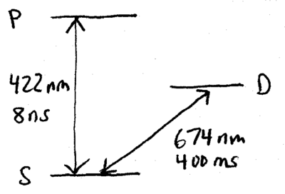
Such experiments with single quantum systems motivate a description of open quantum system dynamics in terms of statistical averages over single realizations, as illustrated by the following experiment. Consider a single three-level ion, such as strontium, with a ns lifetime nm S-P transition, and a ms lifetime nm S-D transition:
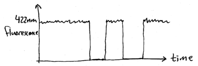
Experimental observation of the blue fluorescence from this atom, when strongly excited at nm, and weakly excited at nm, shows a very interesting signature: quantum jumps. When the atom is in the metastable D state, the nm fluorescence ceases, because no photons can be scattered from the strong transition until it transitions back to the ground S state. A typical observation record might look like this:
Naturally, the average fluorescence rate will be consistent with that expected by the relative strengths of the red and blue excitations, but this would be just a constant value. Such quantum jumps, however, are ubiquitous in experiments involving single atoms and other single quanta, and it would be nice to have a theoretical prescription for describing such observations. In addition, it would be nice to have available possible interpretations of what how the individual systems might be evolving to give some observed ensemble behavior, such as an exponential decay.
Quantum Monte-Carlo wavefunction technique for atom + vacuum
Consider a single two-level atom evolving under the Hamiltonian , while also undergoing spontaneous emission. This is the same scenario we studied to formulate the optical Bloch equations. It can be modeled using the quantum Monte-Carlo wavefunction (QMCWF) technique, using the following steps.
Let us assume the atom begins in some state , and let the atomic levels be and . Let be the decay rate of the excited state, as determined, for example, from Fermi's golden rule. The QMCWF technique introduces a new non-Hermitian "Hamiltonian"
which governs evolution of the state, according to the following. For each differential time step , the state evolves as:
- 1. Compute
- 2. Let be a uniformly distributed random number
- 3. If then
- 4. If then
- 5. Go to 1
Physically, is the probability of the atom jumping from to , that is, spontaneously emitting a photon, during the time interval . Note that typically , and
so is the normalization of the state after of evolution under the non-Hermitian Hamiltonian . Essentially, the QMCWF scheme models an imaginary observer watching for a spontaneously emitted photon coming from the atom. If a photon is emitted, then the atom transitions immediately into ; this is the rule given in step 3, and such a transition is known as a quantum jump. Otherwise, if no photon is emitted, the state changes nevertheless, albeit by only a small amount. Because the observer saw no photon, and thus the probability of the atom being in is slightly diminished. Specifically, if , and , then according to the rule in step 4,
This is exactly the same physics we have seen earlier, in the beamspliter model of the optical Bloch equations.
Equivalence of QMCWF and the optical Bloch equations
The equivalence of QMCWF and the optical Bloch equations (OBE) is shown by demonstrating that the evolution of the density matrix
satisfies the OBE, where the average (denoted by the overline) is taken over instances of running the QMCWF procedure. This follows from computing the density matrix for the state after one QMCWF procedure step:
Writing this as a coarse-grained differential equation, taking the limit of small , we find
This is the optical Bloch equation.
Quantum Monte-Carlo wavefunction technique: general case
The method of the quantum Monte-Carlo wavefunction technique can be applied not just to the atom + vacuum scenario, but also to model any open quantum system dynamics. The relaxation part of a master equation may be described by a Lindblad operator
where are known as "quantum jump" operators. The corresponding QMCWF procedure employs the non-Hermitian Hamiltonian
and the steps
- 1. Compute , and
- 2. Let be a uniformly distributed random number
- 3. If then with randomly chosen with probability .
- 4. If then
- 5. Go to 1
There are some computational advantages to the QMCWF approach, over numerical solution of the differential equations normally obtained with master equations. In particular, an dimensional Hilbert space described by a density matrix requires variables, whereas a pure-state wavefunction requires only variables. Of course, calculating expectation values means that the stochastic evolution of the QMCWF technique must be repeated times, so the overall effect is a tradeoff between storage space and computational time. However, the QMCWF technique is immediately parallelizable, and often (but not always) desired observables converge quickly.
For more about this, see, for example, the nice article <refbase>5239</refbase> by Molmer, Castin, and Dalibard, "Monte Carlo wave-function method in quantum optics", J. Opt. Soc. Am. B, v10, p524, 1993. --> http://www.opticsinfobase.org/abstract.cfm?URI=josab-10-3-524. See also by the same authors --> http://prl.aps.org/pdf/PRL/v68/i5/p580_1.
Example: spontaneous emission
The dynamics of an atom interacting with the vacuum can be described not just by the usual optical Bloch equations, but also, by an infinite variety of alternate pictures. This can be seen through a simple example using the quantum monte-carlo wavefunction technique.
Let , , and denote the Pauli matrices, as usual. Recall that the optical Bloch equations
can be written as
using
In the "standard" unraveling of spontaneous emission into quantum jumps, in the absence of a classical driving field, there is no Hamiltonian evolution () and one jump operator, . This gives exactly the standard optical Bloch equations, as was seen above. Unraveling the dynamics with the quantum monte carlo wavefunction technique, we obtain evolution trajectories which look like this:
<youtube>0UfqGc0NUCc</youtube>
The average over many such evolutions leads to the exponential decay expected from the optical Bloch equations:
<youtube>8ErLH7LGYqM</youtube>
An alternate unraveling of spontaneous emission
However, it turns out that identical dynamics are obtained, on average, with the same form of master equation, but with and , instead.
<youtube>BLOZnYN2rDw</youtube>
The average over many such evolutions also leads to the exponential decay expected from the optical Bloch equations:
<youtube>F8xHZ4KHvS8</youtube>
Analytically, the exact agreement can be proven by writing the master equation as a set of differential equations for , with the alternate choice of and .
The origin of this alternate unraveling of spontaneous emission arises in the lack of knowledge about what basis the environment is observing the system in, as can be seen in the discussion about another representation of open quantum system dynamics, the operator sum representation.
Example: phase and amplitude damping
Spontaneous emission, which is mainly what we have studied so far, with the OBE and QMCWF, is described by the density matrix evolution
Here, is the spontaneous emission rate of the atom, parameterizing the loss of energy from the atom (the decay of the diagonal elements of to ), and the simultaneous loss of phase coherence of the atom (the decay of the off-diagonal elements of to zero). The quantum jump operator for spontaneous emission, in a two-level atom, is . More generally, however, we can have two parameters which describe separate decay of the diagonal and off-diagonal elements,
where is the energy loss rate, and is the rate of loss of quantum coherence, also known as the phase damping rate. Both of these effects are known as decoherence.
In particular, we define decoherence as any process which can turn pure states into statistical mixtures. A density matrix is pure if either , or for some state , or the entropy . Otherwise, it is mixed.
Phase damping, which gives rise to , is in a sense the most "quantum" kind of noise; it comes along with spontaneous emission, but can also exist by itself. Historically, the term "decoherence" has sometimes been identified exclusively with phase damping, because of its important role in the emergence of classical behavior from quantum systems, but today, decoherence is used as a much more general term, because there are so many ways to lose coherence from a quantum system other than just phase damping.
Open system dynamics have infinitely many equivalent unravelings
The various physical origins of phase damping are interesting to consider, because they can teach us an important fact about models of decoherence for single quantum systems: just as can be unraveled in infinitely many ways as , decoherence processes may also be unraveled in an infinite number of ways, each equally equivalent and equally physically meaningful.
We consider three different physical models of phase damping, on a two-level atom.
Random phase noise
A two-level atom of frequency excited by far off-resonance light, , experiences an AC stark shift of amount proportional to the light intensity. If this intensity fluctuates, then the atom's phase is randomly modulated, causing the evolution
(6.2.1)
where is the phase imparted by the AC stark shift. Suppose is modeled as a Gaussian distributed random variable, with mean zero and variance , such that
If the initial state of the atom is , then after time , it evolves into the average state described by the density matrix
which is found to be
(6.2.2)
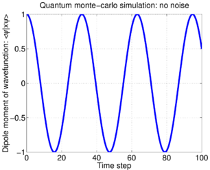
If the atomic Hamiltonian is , and the atom's initial state is , then the dipole moment of the atom shows a simple Rabi oscillation:
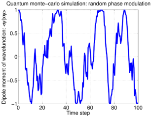
When random phase noise is imposed on the atom, then its dipole moment decays with time. The evolution of a single atom, according to the "trajectory" described by the random walk of Eq.(6.2.1), is a noisy Rabi oscillation:
Here is an animation of seven sample trajectories, which makes it clear that the average of all these evolutions produces an exponential decay, due to the random phase jitter between the trajectories:
<youtube>rNPbL_xl8ag</youtube>
Elastic collisions
Another physical origin for phase damping is elastic collisions. Assume the two-level atom bounces along a waveguide, interacting with the walls without loosing kinetic energy, but changing its trajectory slightly at each bounce, in a manner depending on the state of the atom. This can be modeled by a Hamiltonian interacting the atom with a single mode environment,
with coupling constant . During a small differential timestep , an initial atomic state coupled to an environment evolves to become
(6.2.3)
where . This expression is very similar to that obtained for the gedankenexperiment used in the QMCWF model of spontaneous emission; the difference is that when a photon is observed in the environment, the atom does not collapse into , but rather, into . In other words, it does not lose energy; it only loses information about what state it was in, prior to the collapse.
Just as in the proof of the equivalence of QMCWF to the OBE, we can compute the density matrix evolution which this model gives rise to, by writing down an expression for , based on Eq.(6.2.3),
Note that this is exactly the same evolution as we obtained for the random phase noise model, Eq.(6.2.2).
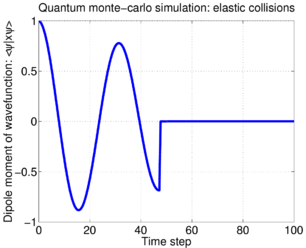
Despite the density matrix evolution being identical to that of the random phase model, the elastic collision model implies a different single-particle evolution trajectory. In contrast to the noisy Rabi oscillations previously seen, for the elastic collisions, the atomic state initially decays, then jumps into the state at some random time; this is illustrated by this sample trajectory:
Again, here is an animation of seven sample trajectories:
<youtube>tpjMZ8hVg-0</youtube>
Phase flips
A third physical model for phase damping is based on quantum jumps. The Lindblad operator for phase damping is evidently
Equivalently, it may be rewritten in standard form as
where
Note that is proportional to the identity, and thus , such that no evolution occurs due to this relaxation process except when a quantum jump occurs. Moreover, the effect of a quantum jump is to flip the phase of the atom by , changing . If such a flip happens with probability at each moment in time, then the density matrix for this evolution is thus
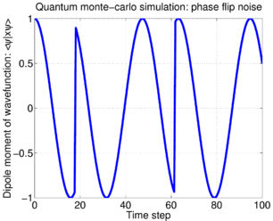
This is again the same density matrix dynamics as previously obtained for the random phase noise and elastic collision models. However, the trajectories of individual evolutions is different; at each moment in time, the two-level atom either remains completely unchanged, or its excited state flips sign, inverting its dipole moment:
Again, here is an animation of seven sample trajectories:
<youtube>uPadYAzgbNM</youtube>
Discussion
We have seen three models of phase damping, all of which produce the same density matrix evolution, but each of which has very different microscopic trajectories for individually evolving systems. Which is correct?
The answer is that all of them are correct, and yet none are. Any of the three can be used for physical intuition and interpretation, but only as long as the only conclusions drawn depend on statistical averages. In fact, in the absence of control over the environment, no experiment can distinguish between phase damping processes described by these three models, even in principle. This strong statement arises from the fact that there are an infinite number of ways a (mixed) density matrix can be written as a statistical mixture of pure states; correspondingly, there are an infinite number of "unravelings" of density matrix time evolutions, into statistical evolutions of pure state wavefunctions.
The freedom of interpretation which arises in studying decoherence processes arises from a unitary degree of freedom. For example, in the QMCWF model, a gedankenexperiment is performed, in which the atom is allowed to decay and the emitted photon is captured. The evolution of the atom cannot depend on what measurement basis is used for the photodetection. This basis choice is a unitary transform which can be chosen arbitrarily in the gedankenexperiment, and different choices lead to the different unravelings of the master equation into trajectories.
References
- <refbase>5239</refbase>
- <refbase>5249</refbase>
- <refbase>5250</refbase>
- <refbase>5251</refbase>




![{\displaystyle |\psi \rangle \leftarrow \left[{e^{-iHdt}/{\sqrt {1-dp}}}\right]|\psi {\rangle }}](https://wikimedia.org/api/rest_v1/media/math/render/svg/ea38bb19eba003090c5ea2fc4753bc4cd31df52b)


![{\displaystyle {\begin{array}{rcl}\rho (t+dt)&=&dp\,|g\rangle \langle g|+(1-dp){\frac {e^{-iHdt}|\psi {\rangle }{\langle }\psi |e^{+iH^{\dagger }dt}}{1-dp}}\\&\approx &dp\,|g\rangle \langle g|+(1-iHdt)\rho (t)(1+iH^{\dagger }dt)\\&\approx &dp\,|g\rangle \langle g|+\rho (t)-i(H\rho (t)-\rho (t)H^{\dagger })dt\\&=&\Gamma dt\langle e|\rho (t)|e\rangle \,|g\rangle \langle g|+\rho (t)-i(H\rho (t)-\rho (t)H^{\dagger })dt\\&=&\Gamma dt|g\rangle \langle e|\rho (t)|e\rangle \langle g|+\rho (t)-idt\left[H_{0},\rho (t)\right]-{\frac {\Gamma }{2}}dt\left(|e\rangle \langle e|\rho (t)+\rho (t)|e\rangle \langle e|\right)\,.\end{array}}}](https://wikimedia.org/api/rest_v1/media/math/render/svg/1ba436928dde0bfd6ab961c25becb6271b29ea26)
![{\displaystyle {\begin{array}{rcl}{\frac {d}{dt}}\rho (t)&\approx &{\frac {\rho (t+dt)-\rho (t)}{dt}}\\&=&-i\left[H_{0},\rho (t)\right]-{\frac {\Gamma }{2}}\left(|e\rangle \langle e|\rho (t)+\rho (t)|e\rangle \langle e|\right)+\Gamma |g\rangle \langle e|\rho (t)|e\rangle \langle g|\,.\end{array}}}](https://wikimedia.org/api/rest_v1/media/math/render/svg/9ce2544d1229c8e30de802c726ebf316608f75b1)


![{\displaystyle {\dot {\rho }}=-{\frac {i}{\hbar }}[H,\rho ]+\left[{L\rho L^{\dagger }-{\frac {1}{2}}(L^{\dagger }L\rho +\rho L^{\dagger }L)}\right]}](https://wikimedia.org/api/rest_v1/media/math/render/svg/6a0a6a9b7d083ab8a39a057bbd85b49e50d257db)
![{\displaystyle {\dot {\vec {r}}}=\left[{\begin{array}{ccc}{-\Gamma /2}&{0}&{0}\\{0}&-\Gamma /2&0\\0&0&-\Gamma \end{array}}\right]{\vec {r}}-\left[{\begin{array}{c}0\\0\\\Gamma \end{array}}\right]\,,}](https://wikimedia.org/api/rest_v1/media/math/render/svg/5121f9c9430497018fbb9615b50437b20574faac)


![{\displaystyle \rho (t=0)=\left[{\begin{array}{cc}{1-c}&{b^{*}}\\{b}&{c}\end{array}}\right]\longrightarrow \rho (t)=\left[{\begin{array}{cc}{1-ce^{-\Gamma t}}&{b^{*}e^{-\Gamma t/2}}\\{be^{-\Gamma t/2}}&{ce^{-\Gamma t}}\end{array}}\right]\,.}](https://wikimedia.org/api/rest_v1/media/math/render/svg/c1ee27d1b27e629da54332593918caec423edb03)


![{\displaystyle \rho (t)=\left[{\begin{array}{cc}{1-ce^{-t/T_{1}}}&{b^{*}e^{-t/T_{2}}}\\{be^{-t/T_{2}}}&{ce^{-t/T_{1}}}\end{array}}\right]\,,}](https://wikimedia.org/api/rest_v1/media/math/render/svg/b44d1f145a6f591cf3c5954d9cc7127aa8d4e973)


![{\displaystyle \rho (t)=\int _{-\infty }^{+\infty }\left[{\begin{array}{cc}{|a|^{2}}&{ab^{*}e^{i\theta }}\\{a^{*}be^{-i\theta }}&{|b|^{2}}\end{array}}\right]{\rm {prob}}(\theta )\,d\theta \,,}](https://wikimedia.org/api/rest_v1/media/math/render/svg/fc4ce9e1acf7b2aeb1b22f032ec0e40947624e5f)
![{\displaystyle \rho (t)=\left[{\begin{array}{cc}{|a|^{2}}&{ab^{*}e^{-\lambda t}}\\{a^{*}be^{-\lambda t}}&{|b|^{2}}\end{array}}\right]\,.}](https://wikimedia.org/api/rest_v1/media/math/render/svg/73319854b548b1a587d1d304dc47cef4b1c64527)


![{\displaystyle H_{SE}=|e\rangle \langle e|\otimes \left[{\gamma |0\rangle \langle 1|+\gamma ^{*}|1\rangle \langle 0|}\right]\,,}](https://wikimedia.org/api/rest_v1/media/math/render/svg/e90891a0247a3396fbb289e6bd7b8a99863381d5)


![{\displaystyle {\begin{array}{rcl}(a|g\rangle +b|e\rangle )\otimes |0{\rangle }&\rightarrow &a|g{\rangle }|0\rangle +b|e\rangle (\cos \theta |0\rangle +\sin \theta |1\rangle )\\&=&\left[{a|g\rangle +b\cos \theta |e\rangle }\right]|0{\rangle }+\left[{b\sin \theta |e\rangle }\right]|1{\rangle }\,,\end{array}}}](https://wikimedia.org/api/rest_v1/media/math/render/svg/971bd5b61c497747a826d480cbf16c3ff9ecfe19)


![{\displaystyle {\begin{array}{rcl}\rho (t)&=&\left[{a|g\rangle +b\cos \theta |e\rangle }\right]\left[{\langle g|a^{*}+\langle e|b^{*}\cos \theta }\right]+|b|^{2}\sin ^{2}\theta |e\rangle \langle e|\\&=&\left[{\begin{array}{cc}{|a|^{2}}&{ab^{*}e^{-\lambda t}}\\{a^{*}be^{-\lambda t}}&{|b|^{2}}\end{array}}\right]\,.\end{array}}}](https://wikimedia.org/api/rest_v1/media/math/render/svg/a91ec6cdace1485c3f2dfcf824e29a06ddd34844)
![{\displaystyle {\mathcal {L}}(\rho )=-{\frac {1}{T_{2}}}\left[{|e\rangle \langle e|\rho |g\rangle \langle g|+|g\rangle \langle g|\rho |e\rangle \langle e|}\right]\,.}](https://wikimedia.org/api/rest_v1/media/math/render/svg/14df0ebf4581b0c47b87a58a479d21059d98c2ae)
![{\displaystyle {\mathcal {L}}(\rho )=-{\frac {1}{2}}\left[{C^{\dagger }C\rho +\rho C^{\dagger }C}\right]+C\rho C^{\dagger }\,,}](https://wikimedia.org/api/rest_v1/media/math/render/svg/b7302feeaf6960b521c8b53a8a80e39e2a1f0be3)
![{\displaystyle C={\frac {1}{\sqrt {2T_{2}}}}\left[{|g\rangle \langle g|-|e\rangle \langle e|}\right]\,.}](https://wikimedia.org/api/rest_v1/media/math/render/svg/ca89e3f0895cc459c05a305631bb213da3410af4)


![{\displaystyle {\begin{array}{rcl}\rho (t)&=&{\frac {1+e^{-\lambda t}}{2}}\left[{a|g\rangle +b|e\rangle }\right]\left[{\langle g|a^{*}+\langle e|b^{*}}\right]+{\frac {1-e^{-\lambda t}}{2}}\left[{a|g\rangle -b|e\rangle }\right]\left[{\langle g|a^{*}-\langle e|b^{*}}\right]\\&=&\left[{\begin{array}{cc}{|a|^{2}}&{ab^{*}e^{-\lambda t}}\\{a^{*}be^{-\lambda t}}&{|b|^{2}}\end{array}}\right]\,.\end{array}}}](https://wikimedia.org/api/rest_v1/media/math/render/svg/d911c6ba1f0d48c0616c85ef91d9637af7712495)
